Identifying viral contigs in metagenomic data
Objectives
- Identifying viral contigs
- Identifying viral contigs using
VirSorter2 - Checking quality and estimating completeness of the viral contigs via
CheckV - Exercise: Examining viral output files from
VirSorter2andCheckV - Introduction to
vConTACT2for predicting taxonomy of viral contigs - OPTIONAL: Visualising the
vConTACT2gene-sharing network inCytoscape
Identifying viral contigs
Viral metagenomics is a rapidly progressing field, and new software are constantly being developed and released each year that aim to better identify and characterise viral genomic sequences from assembled metagenomic sequence reads.
Currently, the most commonly used methods are VirSorter2, VIBRANT, and VirFinder (or the machine learning implementation of this, DeepVirFinder). A number of recent studies use one of these tools or a combination of several at once.
Uses a predicted protein homology reference database-based approach, together with searching for a number of pre-defined metrics based on known viral genomic features. VirSorter2 includes dsDNAphage, ssDNA, and RNA viruses, and the viral groups Nucleocytoviricota and lavidaviridae.*
More info
Uses a machine learning approach based on protein similarity (non-reference-based similarity searches with multiple HMM sets), and is in principle applicable to bacterial and archaeal DNA and RNA viruses, integrated proviruses (which are excised from contigs by VIBRANT), and eukaryotic viruses.
More info
Uses a machine learning based approach based on k-mer frequencies. Having developed a database of the differences in k-mer frequencies between prokaryote and viral genomes, VirFinder examines assembled contigs and identifies whether their k-mer frequencies are comparable to known viruses in the database, using this to predict viral genomic sequence. This method has some limitations based on the viruses that were included when building the database (bacterial DNA viruses, but very few archaeal viruses, and, at least in some versions of the software, no eukaryotic viruses). However, tools are also provided to build your own database should you wish to develop an expanded one. Due to its distinctive k-mer frequency-based approach, VirFinder may also have the capability of identifying some novel viruses overlooked by tools such as VIBRANT or VirSorter.
More info
Identifying viral contigs using VirSorter2
For this exercise, we will use VirSorter2 to identify viral contigs from our assembled contigs. We can also use VirSorter2 to prepare files for later use with the gene annotation tool DRAM-v, which we'll run later in the day.
Checking quality and estimate completeness of the viral contigs via CheckV
CheckV was developed as an analogue to CheckM. CheckV first performs a 'contaminating sequence' trim, removing any retained (prokaryote) host sequence on the end of contigs with integrated prophage, and then assesses the quality and completeness of the assembled viral contigs. The quality of the contigs are also categoriesed based on the recently developed Minimum Information about an Unclutivated Virus Genome (MIUViG) standards for reporting sequences of unclutivated virus geneomes (such as those recovered from metagenomic sequencing data). The MIUViG were developed as an extension of the Minimum Information about any (x) Sequence (MIxS) standards, which include, among others, standards for Metagenome-Assembled Genomes (MIMAG).
Run VirSorter2 and CheckV
These exercises will take place in the 7.viruses/ folder.
For VirSorter2, we will input the assembled contigs from the SPAdes assembly we performed earlier. These assembly files have been copied to 7.viruses/spades_assembly/ for this exercise.
We will then run CheckV in the same script, providing the FASTA file of viral contigs output by VirSorter2 as input (final-viral-combined.fa).
Remember to update <YOUR FOLDER> to your own folder.
code
module unload XALT
For the VirSorter/2.2.3-gimkl-2020a-Python-3.8.2 NeSI module to work properly, we must also include module unload XALT in the script above.
VirSorter2 parameters
The key parameters you may want to consider altering for your own work are --min-score and --include-groups. For today's excersice we will include all available groups (--include-groups dsDNAphage,NCLDV,RNA,ssDNA,lavidaviridae), and will set the min-score to 0.7. You can expiriment with this value for your own data (see the Virsorter2 github page for more information).
VirSorter2 for your own work
The required databases for VirSorter2 are not loaded with the NeSI module. For your own work, you will need to first download these databases and provide the path to the -d flag below. For today's workshop this is already set up.
Outputs of VirSorter2 and CheckV
Key outputs from VirSorter2 include:
mgss-final-viral-combined.fa: FASTA file of identified viral sequencesmgss-final-viral-score.tsv: table with score of each viral sequences across groups and a few more key features, which can also be used for further filteringmgss-for-dramv/: files to be used as input toDRAM-vfor gene prediction and annotation (we will be runningDRAM-vlater today during the gene annotation session)
CheckV provides summary outputs for contamination, completeness, repeats, and an overall quality summary. Later today we will have a brief look at some examples of the information you can draw from these CheckV outputs.
Exercise: Examining viral output files from VirSorter2 and CheckV
VirSorter2 and CheckV provide several of different output files that are important for identifying and understanding the viruses present in your data. Explore through the following files:
7.viruses/VirSorter2/mgss-final-viral-score.tsv7.viruses/checkv_out/quality_summary.tsv
When viewing these files, see if you can find the following information:
- How many viral contigs did
VirSorter2identify? - How many viral contigs meet the "High-quality" (MIUViG) standard?
- How many might we consider "complete" genomes based on
CheckV's completeness estimation? - Are any of the identified viral contigs complete circular genomes (based on identifying direct terminal repeat regions on both ends of the genome)? If not, think about why this might be the case for this dataset (hint: the workshop materials are a manufactured "metagenome" data set based on compiling several individual genomes)
- Are there any suspicious contigs that you might want to flag for closer examination (and/or careful consideration in downstream analyses)? (Note that standard practice would be to use these
CheckVresults as one basis for filtering to remove potential false positives)
Introduction to vConTACT2 for predicting taxonomy of viral contigs
Even more so than prokaryote taxonomy, establishing a coherent system for viral taxonomy is complex and continues to evolve. In 2020, the International Committee on Taxonomy of Viruses (ICTV) overhauled the classification code into 15 hierarchical ranks. Furthermore, the knowledge gap in databases of known and taxonomically assigned viruses remains substantial, and so identifying the putative taxonomy of viral contigs from environmental metagenomics data remains challenging.
There are a number of approaches that can be used to attempt to predict the taxonomy of the set of putative viral contigs output by programs such as VIBRANT, VirSorter, and VirFinder. vConTACT2 is one such method that uses 'guilt-by-contig-association' to predict the potential taxonomy of viral genomic sequence data based on relatedness to known viruses within a reference database (such as viral RefSeq). The principle is that, to the extent that the 'unknown' viral contigs cluster closely with known viral genomes, we can then expect that they are closely related enough to be able to predict a shared taxonomic rank.
Note
Anecdotally, however, in my own experience with this process I have unfortunately been unable to directly predict the taxonomy of the vast majority of the viral contigs output by VIBRANT, VirSorter, or VirFinder from an environmental metagenomic data set (due to not clustering closely enough with known viruses in the reference database). You can, however, visualise the gene-sharing network generated to infer the likely taxonomy of each of your viruses at higher taxonomic ranks due to the relatedness to known reference viral genomes.
Running vConTACT2 can require a considerable amount of computational resources, and so we won't be running this in the workshop today. The required process is outlined for reference in an Appendix for this exercise, should you wish to experiment with this on your own data in the future.
For today, we have provided some of the output files from this process when applied to our mock metagenome data. A selection of these can be viewed in the folder 7.viruses/vConTACT2_Results/ via head or less.
A few notes to consider:
- You will see that the
genome_by_genome_overview.csvfile contains entries for the full reference database used as well as the input viral contigs (contigs starting withNODE). -
You can use a command such as
grep "NODE" vConTACT2_Results/genome_by_genome_overview.csv | lessto view only the lines for the input contigs of interest.- Note also that these lines however will not contain taxonomy information.
- See the notes in the Appendix for further information about why this might be.
-
As per the notes in the Appendix, the
tax_predict_table.tsvfile contains predictions of potential taxonomy (and or taxonomies) of the input viral contigs for order, family, and genus, based on whether they clustered with any viruses in the reference database.- Note that these may be lists of multiple potential taxonomies, in the cases where viral contigs clustered with multiple reference viruses representing more than one taxonomy at the given rank.
The taxonomies are deliberately enclosed in square brackets (
[ ]) to highlight the fact that these are predictions, rather than definitive taxonomy assignments.
(Optional) Visualising the vConTACT2 gene-sharing network in Cytoscape
We can visualise the gene-sharing network generated by vConTACT2 (c1.ntw) using the software Cytoscape. Cytoscape runs as a GUI (graphical user interface), so we will need to either download and install this software or open Cytoscape using NeSI's Virtual Desktop (instructions can be found here). With our Virtual Desktop open, Cytoscape can then be loaded as follows.
Copy/paste in the Virtual Desktop
You will not be able to copy text from outside the Virtual Desktop and paste into the Virtual Desktop, in which case you will need to manually type these commands.
Open a terminal in Virtual Desktop prior to running code below
Do not update Cytoscape!
A dialog box will appear telling you about a new version of Cytoscape. Click "close", as we will not be installing any new versions today!
Load the network
- With
Cytoscapeopen, click on File \(\rightarrow\) Import \(\rightarrow\) Network from file - Open the
c1.ntwfile by (a) typing in the absolute path in the File Name box:/nesi/nobackup/nesi02659/MGSS_U/<YOUR FOLDER>/7.viruses/vConTACT2_Results/c1.ntwor (b) navigate to the file using the GUI. -
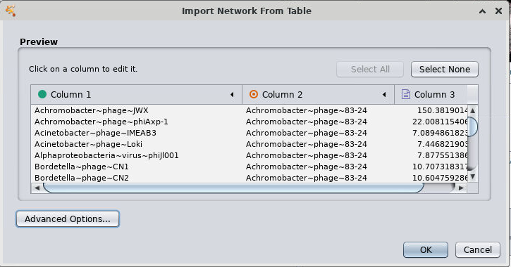
In the Import Network From Table pop-up box:
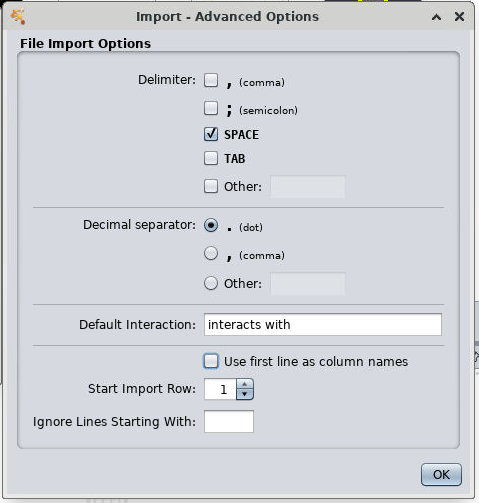
- Click on Advanced Options
- Select SPACE as the delimiter
- Uncheck Use first line as column names
- Click OK
- In the drop-down menu for 'Column 1', select the green dot (source node)
- For Column 2 select the red target (Target node)
- Click OK
- Click on Advanced Options
It will now ask if you want to create a view for your large networks now. Click OK. This may take a minute to generate the network visualisation.
Annotate the network
There are many ways to modify and inspect this visualisation. One basic addition that will help us interpret the results here is to colour code the viral genomes based on reference (RefSeq) genomes and the viral contigs recovered from our dataset. We can do this by loading the genome_by_genome_overview.csv file.
Dataset column
For the purposes of this workshop, we have added the additional column Dataset to the genome_by_genome_overview.csv file stating whether each viral sequence originated from either the reference database (RefSeq) or our own data (Our_data). This column is not generated by vConTACT2, but you can open the file in Excel to add any additional columns you would like to colour code the nodes by.
Click File/Import/Table from file and select the genome_by_genome_overview.csv file to open. In the pop-up box, leave the settings as default and click OK. This will add a bunch of metadata to your network table. We can now use this to colour code the nodes in the network.
To colour code the nodes by genome source (Refseq or Our_data):
- Click the
Styletab on the far left - Select the dropdown arrow by
Fill Color - Next to
Columnclick on --select value-- and selectDataset - For
Mapping Type, selectDiscrete Mapping. - Then for each of
RefseqandOur_data, click the three dots in the empty box to the right of the label and select a colour for that dataset.
You can now zoom in on the network and select viral contigs from your own dataset, and examine which reference viruses may be the most closely related. This can give an indication of the possible taxonomy of your own viruses based on their gene-sharing relatedness to the known reference genomes.