Gene annotation II: DRAM and coverage calculation

Objectives

• Gene prediction and annotation with DRAM
• Annotating MAGs with DRAM
• Annotating viral contigs with DRAM-v
• Calculating per-sample coverage stats for prokaryotic bins
• Calculating per-sample coverage stats for viral contigs
• Select initial goal

---

Gene prediction and annotation with DRAM (Distilled and Refined Annotation of Metabolism)

DRAM is a tool designed to profile microbial (meta)genomes for metabolisms known to impact ecosystem functions across biomes. DRAM annotates MAGs and viral contigs using KEGG (if provided by user), UniRef90, PFAM, CAZy, dbCAN, RefSeq viral, VOGDB (Virus Orthologous Groups), and the MEROPS peptidase database. It is also highly customizable to other custom user databases.

DRAM only uses assembly-derived FASTA files input by the user. These input files may come from unbinned data (metagenome contig or scaffold files) or genome-resolved data from one or many organisms (isolate genomes, single-amplified genome (SAGs), MAGs).

DRAM is run in two stages: annotation and distillation.

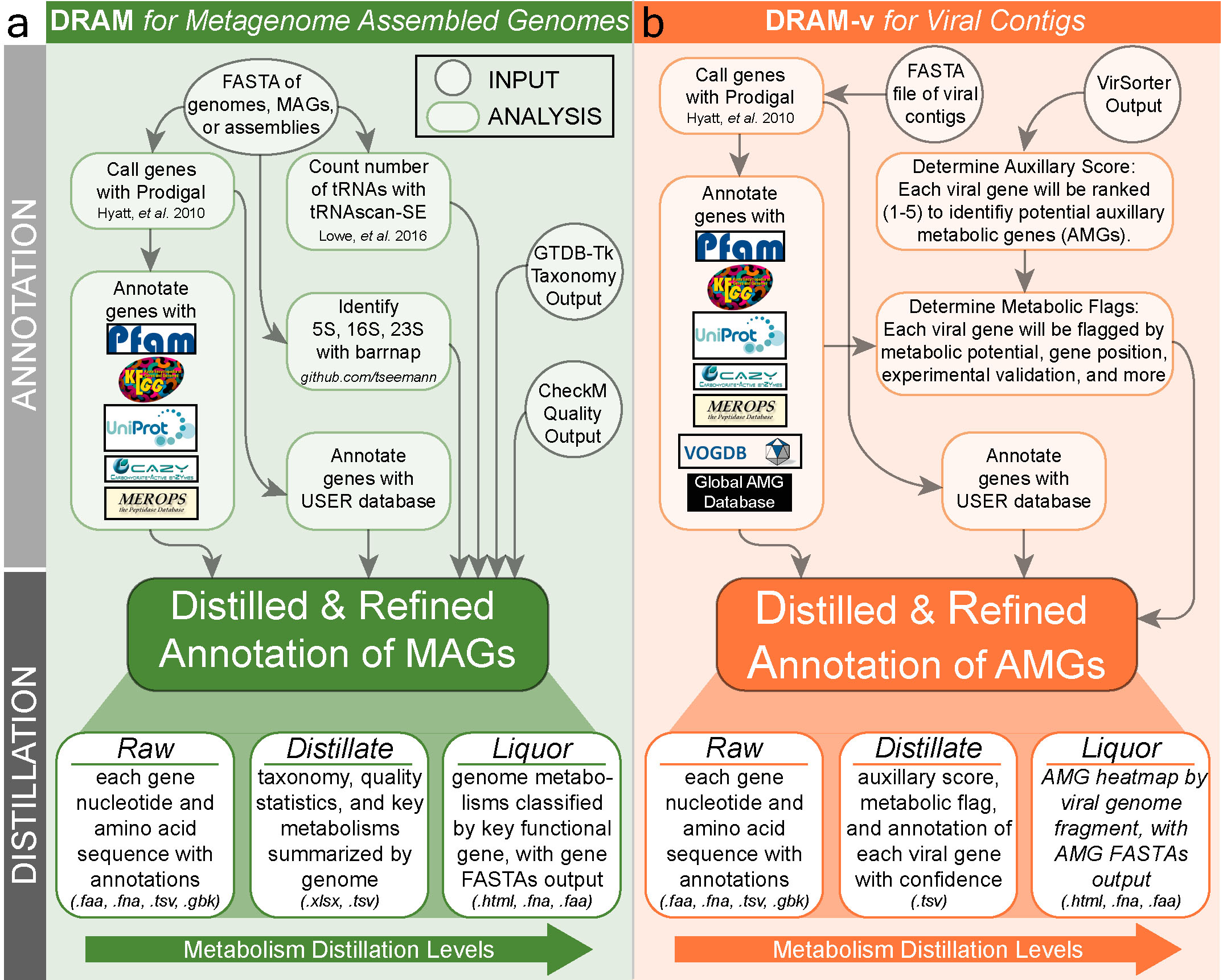
1. Annotation

The first step in DRAM is to annotate genes by assigning database identifiers to genes. Short contigs (default < 2,500 bp) are initially removed. Then, Prodigal is used to detect open reading frames (ORFs) and to predict their amino acid sequences. Next, DRAM searches all amino acid sequences against multiple databases, providing a single Raw output. When gene annotation is complete, all results are merged in a single tab-delimited annotation table, including the best hit for each database for user comparison.

2. Distillation

After genome annotation, a distill step follows with the aim to curate these annotations into useful functional categories, creating genome statistics and metabolism summary files, which are stored in the Distillate output. The genome statistics provides most genome quality information required for MIMAG standards, including GTDB-tk and CheckM information if provided by the user. The summarised metabolism table includes the number of genes with specific metabolic function identifiers (KO, CAZY ID, etc) for each genome, with information obtained from multiple databases. The Distillate output is then further distilled into the Product, an html file displaying a heatmap, as well as the corresponding data table. We will investigate all these files later on.

---

Annotating MAGs with DRAM

Beyond annotation, DRAM aims to be a data compiler. For that reason, output files from both CheckM and GTDB_tk steps can be input to DRAM to provide both taxonomy and genome quality information of the MAGs.

DRAM input files

For these exercises, we have copied the relevant input files into the folder 10.gene_annotation_and_coverage/DRAM_input_files/. gtdbtk.bac120.summary.tsv was taken from the earlier 8.prokaryotic_taxonomy/gtdbtk_out/ outputs, and filtered_bins_checkm.txt from the result of re-running CheckM on the final refined filtered bins in 6.bin_refinement/filtered_bins.

Navigate to working directory

cd /nesi/nobackup/nesi02659/MGSS_U/<YOUR FOLDER>/10.gene_annotation_and_coverage/

Along with our filtered bins, the CheckM output file (checkm.txt) and GTDB-Tk summary output gtdbtk.bac120.summary.tsv are used as inputs as is.

DRAM annotation

In default annotation mode, DRAM only requires as input the directory containing all the bins we would like to annotate in fastA format (either .fa or .fna). There are few parameters that can be modified if not using the default mode. Once the annotation step is complete, the mode distill is used to summarise the obtained results.

UniRef and RAM requirements

Due to the increased memory requirements, annotations against the UniRef90 database is not set by default and the flag –use_uniref should be specified in order to search amino acid sequences against UniRef90. In this exercise, due to memory and time constraints, we won't be using the UniRef90 database.

We will start by glancing at some of the options for DRAM.

code

module purge
module load DRAM/1.3.5-Miniconda3

DRAM.py --help

Terminal output

usage: DRAM.py [-h] {annotate,annotate_genes,distill,strainer,neighborhoods,merge_annotations} ...

positional arguments:
  {annotate,annotate_genes,distill,strainer,neighborhoods,merge_annotations}
    annotate            Annotate genomes/contigs/bins/MAGs
    annotate_genes      Annotate already called genes, limited functionality compared to annotate
    distill             Summarize metabolic content of annotated genomes
    strainer            Strain annotations down to genes of interest
    neighborhoods       Find neighborhoods around genes of interest
    merge_annotations   Merge multiple annotations to one larger set

options:
  -h, --help            show this help message and exit

To look at some of the arguments in each command, type the following:

code

# DRAM.py <command> --help

# For example:
DRAM.py annotate --help

Submitting DRAM annotation as a slurm job

To run this exercise we first need to set up a slurm job. We will use the results for tomorrow's distillation step.

Create script named annotate_dram.sl

nano annotate_dram.sl

Remember to update <YOUR FOLDER> to your own folder

code

#!/bin/bash -e

#SBATCH --account       nesi02659
#SBATCH --job-name      annotate_DRAM
#SBATCH --partition     milan
#SBATCH --time          5:00:00
#SBATCH --mem           30Gb
#SBATCH --cpus-per-task 24
#SBATCH --error         %x_%A.err
#SBATCH --output        %x_%A.out

# Load modules
module purge
module load DRAM/1.3.5-Miniconda3

# Working directory
cd /nesi/nobackup/nesi02659/MGSS_U/<YOUR FOLDER>/10.gene_annotation_and_coverage

# Run DRAM
DRAM.py annotate -i 'filtered_bins/*.filtered.fna' \
                 --checkm_quality DRAM_input_files/filtered_bins_checkm.txt \
                 --gtdb_taxonomy DRAM_input_files/gtdbtk.bac120.summary.tsv \
                 -o dram_annotations --threads $SLURM_CPUS_PER_TASK

Submit the job

sbatch annotate_dram.sl

The program will take 4-4.5 hours to run, so we will submit the jobs and inspect the results tomorrow morning.

---

Annotating viral contigs with DRAM-v

DRAM also has an equivalent program (DRAM-v) developed for predicting and annotating genes of viral genomes. A number of the options are similar to the standard DRAM run above, although the selection of databases differs slightly, and the subsequent distill step is focussed on identifying and classifying auxilliary metabolic genes (AMGs) rather than the metabolic pathways output by DRAM's standard distill step.

To see more details on options for DRAM-v we can run the same --help command as above:

code

# DRAM-v.py <command> --help

# For example:
DRAM-v.py annotate --help
DRAM-v.py distill --help

Submit DRAM-v annotation as a slurm job

To run this exercise we first need to set up a slurm job. We will use the results for tomorrow's distillation step.

Note

DRAM-v requires the mgss-for-dramv/ files final-viral-combined-for-dramv.fa and viral-affi-contigs-for-dramv.tab that were generated by VirSorter2. These have been copied into 10.gene_annotation_and_coverage/ for this exercise.

Create script named annotate_dramv.sl

nano annotate_dramv.sl

Remember to update <YOUR FOLDER> to your own folder

code

#!/bin/bash -e

#SBATCH --account       nesi02659
#SBATCH --job-name      annotate_DRAMv
#SBATCH --partition     milan
#SBATCH --time          02:00:00
#SBATCH --mem           10Gb
#SBATCH --cpus-per-task 12
#SBATCH --error         %x_%A.err
#SBATCH --output        %x_%A.out

# Load modules
module purge
module load DRAM/1.3.5-Miniconda3

# Working directory
cd /nesi/nobackup/nesi02659/MGSS_U/<YOUR FOLDER>/10.gene_annotation_and_coverage

# Run DRAM-v
DRAM-v.py annotate --threads ${SLURM_CPUS_PER_TASK} \
--min_contig_size 1000 \
-i mgss-for-dramv/final-viral-combined-for-dramv.fa \
-v mgss-for-dramv/viral-affi-contigs-for-dramv.tab \
-o dramv_annotations

Submit the job

sbatch annotate_dramv.sl

We will submit this job now and inspect the results tomorrow morning.

---

Calculating per-sample coverage stats for prokaryotic bins

One of the first questions we often ask when studying the ecology of a system is: What are the pattens of abundance and distribution of taxa across the different samples? With bins of metagenome-assembled genome (MAG) data, we can investigate this by mapping the quality-filtered unassembled reads back to the refined bins to then generate coverage profiles. Genomes in higher abundance in a sample will contribute more genomic sequence to the metagenome, and so the average depth of sequencing coverage for each of the different genomes provides a proxy for abundance in each sample.

As per the preparation step at the start of the binning process, we can do this using read mapping tools such as Bowtie, Bowtie2, and BBMap. Here we will follow the same steps as before using Bowtie2, samtools, and MetaBAT's jgi_summarize_bam_contig_depths, but this time inputting our refined filtered bins.

These exercises will take place in the 10.gene_annotation_and_coverage/ folder. Our final filtered refined bins from the previous bin refinement exercise have been copied to the 10.gene_annotation_and_coverage/filtered_bins/ folder.

First, concatenate the bin data into a single file to then use to generate an index for the read mapper.

Concatenate bin nucleotide FASTA files

cat filtered_bins/*.fna > filtered_bins.fna

Now build the index for Bowtie2 using the concatenated bin data. We will also make a new directory bin_coverage/ to store the index and read mapping output into.

Build Bowtie2 index

mkdir -p bin_coverage/

# Load Bowtie2
module purge
module load Bowtie2/2.4.5-GCC-11.3.0

# Build Bowtie2 index
bowtie2-build filtered_bins.fna bin_coverage/bw_bins

Map the quality-filtered reads (from ../3.assembly/) to the index using Bowtie2, and sort and convert to .bam format via samtools.

Create script named mapping_filtered_bins.sl

nano mapping_filtered_bins.sl

Remember to update <YOUR FOLDER> to your own folder

code

#!/bin/bash -e

#SBATCH --account       nesi02659
#SBATCH --job-name      mapping_filtered_bins
#SBATCH --partition     milan
#SBATCH --time          00:05:00
#SBATCH --mem           1GB
#SBATCH --cpus-per-task 10
#SBATCH --error         %x_%j.err
#SBATCH --output        %x_%j.out

# Load modules
module purge
module load Bowtie2/2.4.5-GCC-11.3.0 SAMtools/1.15.1-GCC-11.3.0

# Working directory
cd /nesi/nobackup/nesi02659/MGSS_U/<YOUR FOLDER>/10.gene_annotation_and_coverage

# Run Bowtie2
for i in {1..4}; do
    bowtie2 --minins 200 --maxins 800 --threads $SLURM_CPUS_PER_TASK --sensitive \
            -x bin_coverage/bw_bins \
            -1 ../3.assembly/sample${i}_R1.fastq.gz \
            -2 ../3.assembly/sample${i}_R2.fastq.gz \
            -S bin_coverage/sample${i}.sam
    samtools sort -@ $SLURM_CPUS_PER_TASK -o bin_coverage/sample${i}.bam bin_coverage/sample${i}.sam
done

Submit the script

sbatch mapping_filtered_bins.sl

Finally, generate the per-sample coverage table for each contig in each bin via MetaBAT's jgi_summarize_bam_contig_depths.

Obtain coverage values

# Load MetaBAT
module load MetaBAT/2.15-GCC-11.3.0

# Calculate coverage table
jgi_summarize_bam_contig_depths --outputDepth bins_cov_table.txt bin_coverage/sample*.bam

The coverage table will be generated as bins_cov_table.txt. As before, the key columns of interest are the contigName, and each sample[1-n].bam column.

Note

Here we are generating a per-sample table of coverage values for each contig within each bin. To get per-sample coverage of each bin as a whole, we will need to generate average coverage values based on all contigs contained within each bin. We will do this in R during our data visualisation exercises on day 4 of the workshop, leveraging the fact that we added bin IDs to the sequence headers.*

Calculating per-sample coverage stats for viral contigs

Here we can follow the same steps as outlined above for the bin data, but with a concatenated FASTA file of viral contigs.

A quick recap

• In previous exercises, we first used VirSorter2 to identify viral contigs from the assembled reads, generating a new fasta file of viral contigs: final-viral-combined.fa
• We then processed this file using CheckV to generate quality information for each contig, and to further trim any retained (prokaryote) sequence on the ends of prophage contigs.

The resultant fasta files generated by CheckV (proviruses.fna and viruses.fna) have been copied to to the 10.gene_annotation_and_coverage/checkv folder for use in this exercise.

Note

Due to the rapid mutation rates of viruses, with full data sets it will likely be preferable to first further reduce viral contigs down based on a percentage-identity threshold using a tool such as BBMap's dedupe.sh or Cluster_genomes_5.1.pl from Simon Roux's group. This would be a necessary step in cases where you had opted for generating multiple individual assemblies or mini-co-assemblies (and would be comparable to the use of a tool like dRep for prokaryote data), but may still be useful even in the case of single co-assemblies incorporating all samples.*

We will first need to concatenate these files together.

code

cat checkv/proviruses.fna checkv/viruses.fna > checkv_combined.fna

Now build the index for Bowtie2 using the concatenated viral contig data. We will also make a new directory viruses_coverage/ to store the index and read mapping output into.

code

mkdir -p viruses_coverage/

# Load Bowtie2
module load Bowtie2/2.4.5-GCC-11.3.0

# Build Bowtie2 index
bowtie2-build checkv_combined.fna viruses_coverage/bw_viruses

Map the quality-filtered reads (from ../3.assembly/) to the index using Bowtie2, and sort and convert to .bam format via samtools.

Create script named mapping_viruses.sl

nano mapping_viruses.sl

Remember to update <YOUR FOLDER> to your own folder

code

#!/bin/bash -e

#SBATCH --account       nesi02659
#SBATCH --job-name      mapping_viruses
#SBATCH --partition     milan
#SBATCH --time          00:05:00
#SBATCH --mem           1GB
#SBATCH --cpus-per-task 10
#SBATCH --error         %x_%j.err
#SBATCH --output        %x_%j.out

# Load modules
module purge
module load Bowtie2/2.4.5-GCC-11.3.0 SAMtools/1.15.1-GCC-11.3.0

# Working directory
cd /nesi/nobackup/nesi02659/MGSS_U/<YOUR FOLDER>/10.gene_annotation_and_coverage

# Run Bowtie2
for i in {1..4}; do
  bowtie2 --minins 200 --maxins 800 --threads $SLURM_CPUS_PER_TASK --sensitive \
            -x viruses_coverage/bw_viruses \
            -1 ../3.assembly/sample${i}_R1.fastq.gz \
            -2 ../3.assembly/sample${i}_R2.fastq.gz \
            -S viruses_coverage/sample${i}.sam
  samtools sort -@ $SLURM_CPUS_PER_TASK -o viruses_coverage/sample${i}.bam viruses_coverage/sample${i}.sam
done

Run the script

sbatch mapping_viruses.sl

Finally, generate the per-sample coverage table for each viral contig via MetaBAT's jgi_summarize_bam_contig_depths.

code

# Load MetaBAT
module load MetaBAT/2.15-GCC-11.3.0

# calculate coverage table
jgi_summarize_bam_contig_depths --outputDepth viruses_cov_table.txt viruses_coverage/sample*.bam

The coverage table will be generated as viruses_cov_table.txt. As before, the key columns of interest are the contigName, and each sample[1-n].bam column.

Note

Unlike the prokaryote data, we have not used a binning process on the viral contigs (since many of the binning tools use hallmark characteristics of prokaryotes in the binning process). Here, viruses_cov_table.txt is the final coverage table. This can be combined with CheckV quality and completeness metrics to, for example, examine the coverage profiles of only those viral contigs considered to be "High-quality" or "Complete".*

Normalise coverage values

Having generated per-sample coverage values, it is usually necessary to also normalise these values across samples of differing sequencing depth. In this case, the mock metagenome data we have been working with are already of equal depth, and so this is an unnecessary step for the purposes of this workshop.

For an example of one way in which the cov_table.txt output generated by jgi_summarize_bam_contig_depths above could then be normalised based on average library size, see the Normalise per-sample coverage Appendix.

---

Select initial goal

It is now time to select the goals to investigate the genomes you have been working with. We ask you to select one of the following goals:

1. Denitrification (Nitrate or nitrite to nitrogen)
2. Ammonia oxidation (Ammonia to nitrite or nitrate)
3. Anammox (Ammonia and nitrite to nitrogen)
4. Sulfur oxidation (SOX pathway, thiosulfate to sulfate)
5. Sulfur reduction (DSR pathway, sulfate to sulfide)
6. Photosynthetic carbon fixation
7. Non-photosynthetic carbon fixation (Reverse TCA or Wood-Ljundahl)
8. Non-polar flagella expression due to a chromosomal deletion
9. Plasmid-encoded antibiotic resistance
10. Aerobic (versus anaerobic) metabolism

Depending on what you are looking for, you will either be trying to find gene(s) of relevance to a particular functional pathway, or the omission of genes that might be critical in function. In either case, make sure to use the taxonomy of each MAG to determine whether it is likely to be a worthwhile candidate for exploration, as some of these traits are quite restricted in terms of which organisms carry them.

To conduct this exersise, you should use the information generated with DRAM as well as the annotation files we created previously that will be available in the directory 10.gene_annotation_and_coverage/gene_annotations.

Please note that we have also provided further annotation files within the directory 10.gene_annotation_and_coverage/example_annotation_tables that contain information obtained after annotating the MAGs against additional databases (UniProt, UniRef100, KEGG, PFAM and TIGRfam). These example files can also be downloaded from here. These files were created by using an in-house python script designed to aggregate different annotations and as part of the environmental metagenomics worflow followed in Handley's lab. Information about using this script as well as the script is available here

---