Assembly evaluation
Objectives
Evaluating the resource consumption of various assemblies
Check to see if your assembly jobs have completed. If you have multiple jobs running or queued, the easiest way to check this is to simply run the squeue command.
Terminal output
If there are no jobs besides your Jupyter session listed, either everything running has completed or failed. To get a list of all jobs we have run in the last day, we can use the sacct command. By default this will report all jobs for the day but we can add a parameter to tell the command to report all jobs run since the date we are specifying.
Terminal output
JobID           JobName          Alloc     Elapsed     TotalCPU  ReqMem   MaxRSS State
--------------- ---------------- ----- ----------- ------------ ------- -------- ----------
38483216        spawner-jupyter+     2    07:45:01     00:00:00      4G          NODE_FAIL
38483216.batch  batch                2    07:45:01     00:00:00                  CANCELLED
38483216.extern extern               2    07:45:01     00:00:00                  CANCELLED
38485254        spades_assembly     12    00:14:38     01:56:40     10G          COMPLETED
38485254.batch  batch               12    00:14:38     01:56:40         7227872K COMPLETED
38485254.extern extern              12    00:14:38     00:00:00                0 COMPLETED
Each job has been broken up into several lines, but the main ones to keep an eye on are the base JobID values.
Using srun
If you use srun, the JobID will have values suffixed with .0. The first of these references the complete job. The later (and any subsequent suffixes like .1, .2) are the individual steps in the script that were called with the srun command.
We can see here the time elapsed for each job, and the number of CPU hours used during the run. If we want a more detailed breakdown of the job we can use the nn_seff command
Terminal output
Here we see some of the same information, but we also get some information regarding how well our job used the resources we allocated to it. You can see here that my CPU and memory usage was somewhat efficient but had high memory efficiency. In the future, I can request less time and retain the same RAM and still had the job run to completion.
CPU efficiency is harder to interpret as it can be impacted by the behaviour of the program. For example, mapping tools like bowtie and BBMap can more or less use all of their threads, all of the time and achieve nearly 100% efficiency. More complicated processes, like those performed in SPAdes go through periods of multi-thread processing and periods of single-thread processing, drawing the average efficiency down.
Evaluating the assemblies using BBMap
Evaluating the quality of a raw metagenomic assembly is quite a tricky process. Since, by definition, our community is a mixture of different organisms, the genomes from some of these organisms assemble better than those of others. It is possible to have an assembly that looks 'bad' by traditional metrics that still yields high-quality genomes from individual species, and the converse is also true.
A few quick checks I recommend are to see how many contigs or scaffolds your data were assembled into, and then see how many contigs or scaffolds you have above a certain minimum length threshold. We will use seqmagick for performing the length filtering, and then just count sequence numbers using grep.
These steps will take place in the 4.evaluation/ folder, which contains copies of our SPAdes and IDBA-UD assemblies.
Remember to update <YOUR FOLDER> to your own folder
code
# Load seqmagick
module purge
module load seqmagick/0.8.4-gimkl-2020a-Python-3.8.2

# Navigate to working directory
cd /nesi/nobackup/nesi02659/MGSS_U/<YOUR FOLDER>/4.evaluation/

# Filter assemblies and check number of contigs
seqmagick convert --min-length 1000 spades_assembly/spades_assembly.fna \
                                    spades_assembly/spades_assembly.m1000.fna
grep -c '>' spades_assembly/spades_assembly.fna spades_assembly/spades_assembly.m1000.fna

seqmagick convert --min-length 1000 idbaud_assembly/idbaud_assembly.fna \
                                    idbaud_assembly/idbaud_assembly.m1000.fna
grep -c '>' idbaud_assembly/idbaud_assembly.fna idbaud_assembly/idbaud_assembly.m1000.fna
Terminal output
If you have your own assemblies and you want to try inspect them in the same way, try that now. Note that the file names will be slightly different to the files provided above. If you followed the exact commands in the previous exercise, you can use the following commands.
code
Choice of software: sequence file manipulation
The tool seqtk is also available on NeSI and performs many of the same functions as seqmagick. My choice of seqmagick is mostly cosmetic as the parameter names are more explicit so it's easier to understand what's happening in a command when I look back at my log files. Regardless of which tool you prefer, we strongly recommend getting familiar with either seqtk or seqmagick as both perform a lot of common FASTA and FASTQ file manipulations.
As we can see here, the SPAdes assembly has completed with fewer contigs assembled than the IDBA-UD, both in terms of total contigs assembled and contigs above the 1,000 bp size. This doesn't tell us a lot though - has SPAdes managed to assemble fewer reads, or has it managed to assemble the sequences into longer (and hence fewer) contigs? We can check this by looking at the N50/L50 (see more information about this statistic here) of the assembly with BBMap.
code
This gives quite a verbose output:
Terminal output
A       C       G       T       N       IUPAC   Other   GC      GC_stdev
0.2541  0.2475  0.2453  0.2531  0.0018  0.0000  0.0000  0.4928  0.0958

Main genome scaffold total:             934
Main genome contig total:               2703
Main genome scaffold sequence total:    34.293 MB
Main genome contig sequence total:      34.231 MB       0.182% gap
Main genome scaffold N/L50:             53/160.826 KB
Main genome contig N/L50:               107/72.909 KB
Main genome scaffold N/L90:             302/15.325 KB
Main genome contig N/L90:               812/4.643 KB
Max scaffold length:                    1.222 MB
Max contig length:                      1.045 MB
Number of scaffolds > 50 KB:            152
% main genome in scaffolds > 50 KB:     77.10%


Minimum         Number          Number          Total           Total           Scaffold
Scaffold        of              of              Scaffold        Contig          Contig
Length          Scaffolds       Contigs         Length          Length          Coverage
--------        --------------  --------------  --------------  --------------  --------
    All                    934           2,703      34,293,018      34,230,627    99.82%
   1 KB                    934           2,703      34,293,018      34,230,627    99.82%
 2.5 KB                    744           2,447      33,967,189      33,909,776    99.83%
   5 KB                    581           2,131      33,379,814      33,328,450    99.85%
  10 KB                    394           1,585      32,031,121      31,994,989    99.89%
  25 KB                    236             916      29,564,265      29,545,757    99.94%
  50 KB                    152             599      26,441,339      26,429,391    99.95%
 100 KB                     92             415      22,238,822      22,230,143    99.96%
 250 KB                     31             153      12,606,774      12,603,418    99.97%
 500 KB                      6              32       4,821,355       4,821,095    99.99%
   1 MB                      1               2       1,221,548       1,221,538   100.00%
N50 and L50 in BBMap
Unfortunately, the N50 and L50 values generated by stats.sh are switched. N50 should be a length and L50 should be a count. The results table below shows the corrected values based on stats.sh outputs.
But what we can highlight here is that the statistics for the SPAdes assembly, with short contigs removed, yielded an N50 of 72.5 kbp at the contig level. We will now compute those same statistics from the other assembly options.
code
| Assembly | N50 (contig) | L50 (contig) |
|---|---|---|
| SPAdes (filtered) | 72.9 kbp | 107 |
| SPAdes (unfiltered) | 72.3 kbp | 108 |
| IDBA-UD (filtered) | 103.9 kbp | 82 |
| IDBA-UD (unfiltered) | 96.6 kbp | 88 |
Reconstruct rRNA using PhyloFlash-EMIRGE
Another method that we can use to obtain taxonomic composition of our metagenomic libraries is to extract/reconstruct the 16S and 18S ribosomal RNA gene. However, modern assemblers often struggle to produce contiguous 16S rRNA genes due to (1) taxa harbouring multiple copies of the gene and (2) repeat regions that short reads cannot span (see here for details). As such, software such as EMIRGE (Miller et al., 2011) and PhyloFlash (Gruber-Vodicka et al., 2020) were developed to reconstruct 16S and 18S rRNA genes. These methods leverage the expansive catalogue of 16S rRNA genes available in databases such as SILVA in order to subset reads and then reconstruct the full-length gene.
For this workshop, we will use PhyloFlash to obtain sequences and abundances of 16S rRNA sequences. The reason being that PhyloFlash can also run EMIRGE as part of its routine, compare those reconstructions with sequences generated by PhyloFlash's map-assemble, and produce a set of 16S rRNA gene sequences as well as estimate relative abundances via coverage estimation.
-lib
A quirk of PhyloFlash is that all outputs will be placed in the current running directory. The only punctuation allowed is "-" and "_". Make sure to name your "LIB" sensibly so you can track which library you're working with.
code
code
A successful run of PhyloFlash (lines 24-29) would have generated the following per-sample outputs:
tar.gzarchive containing relevant data files- An
.htmlpage summary - A timestamped
.logdetailing what was done
The reconstructed 16S rRNA sequences are stored in the per-sample archive. We will extract them to explore the data files inside.
code
The reconstructed sequences based on the phyloFlash and EMIRGE workflows are stored in sample?.phyloFlash/sample?.all.final.fasta.
In lines 32-34 of our slurm script, we also ran a cross-sample comparison script. This generated 4 files:
allsamples_compare.barplot.pdfA relative abundance barplot of identified taxaallsamples_compare.heatmap.pdfA heatmap of identified taxaallsamples_compare.matrix.tsvA dissimilarity matrix (abundance-weighted, UniFrac-like)allsamples_compare.ntu_table.tsv(long/tidy-format table of relative abundance per sample per taxa)
The allsamples_compare.ntu_table.tsv is especially useful if you intend to perform downstream diversity analyses in R.
Sequence taxonomic classification using Kraken2
Most, if not all, of the time, we never know the taxonomic composition of our metagenomic reads a priori. For some environments, we can make good guesses (e.g., Prochlorococcus in marine samples, members of the Actinobacteriota in soil samples, various Bacteroidota in the gut microbiome, etc.). Here, we can use Kraken2, a k-mer based taxonomic classifier to help us interrogate the taxonomic composition of our samples. This is helpful if there are targets we might be looking for (e.g. working hypotheses, well characterised microbiome). Furthermore, we can estimate the abundance of the classified taxa using Bracken.
code
The main output is quite dense and verbose with columns indicated here. The report is more human-readable, with nicely spaced columns that indicate:
- Percentage reads mapped to taxon
- Number of reads mapped to taxon
- Number of reads directly assigned to taxon
- Rank of taxon
- NCBI taxonomy ID
- Scientific name of taxon
Remember to produce the --report as Bracken bases its estimation on the report
The code tells Kraken2 that the inputs ${r1} and ${r1/R1/R2} are paired-end reads. The # after ${base} will be replaced with the read orientation (i.e., forward _1 or reverse _2).
The Bracken outputs provides us with adjusted number (columns added_reads and new_est_reads) and fraction of reads that were assigned to each species identified by Kraken2 for downstream analyses.
Database construction for Kraken2 and Bracken
For this workshop (and most applications), the standard or other extensive pre-built Kraken2 databases are sufficient. However, if you require specific reference sequences to be present, the database building process (outlined here) can be quite time and resource intensive.
The Kraken2 database also comes with a few pre-built Bracken databases (filenames look like this: database100mers.kmer_distrib). Note that the "100mers" doesn't refer to k-mers (oligonucleotide frequency), but it is the length of the read the database was built for. In this workshop, we've used the 100bp database to estimate abundances for 126bp reads. According to the developers, this is acceptable. As long as the read length of the built database is \(\le\) than the length of reads to be classified, Bracken will provide good enough estimates.
If you want to build your own Bracken database based on your library minimum read lengths, you can follow the process here. Take note that you will require the initial sequence and taxonomy files used for building the Kraken2 database (not part of the files in the pre-built databases) and these (especially for NCBI nt and bacterial databses) will take a long time to download and lots of memory to build.
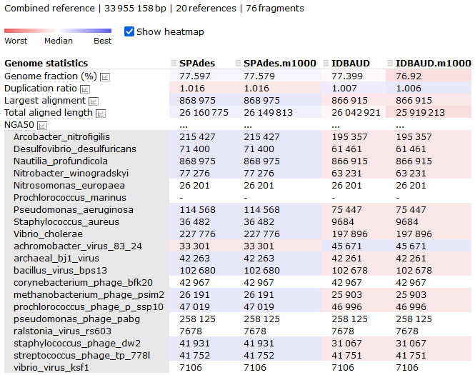
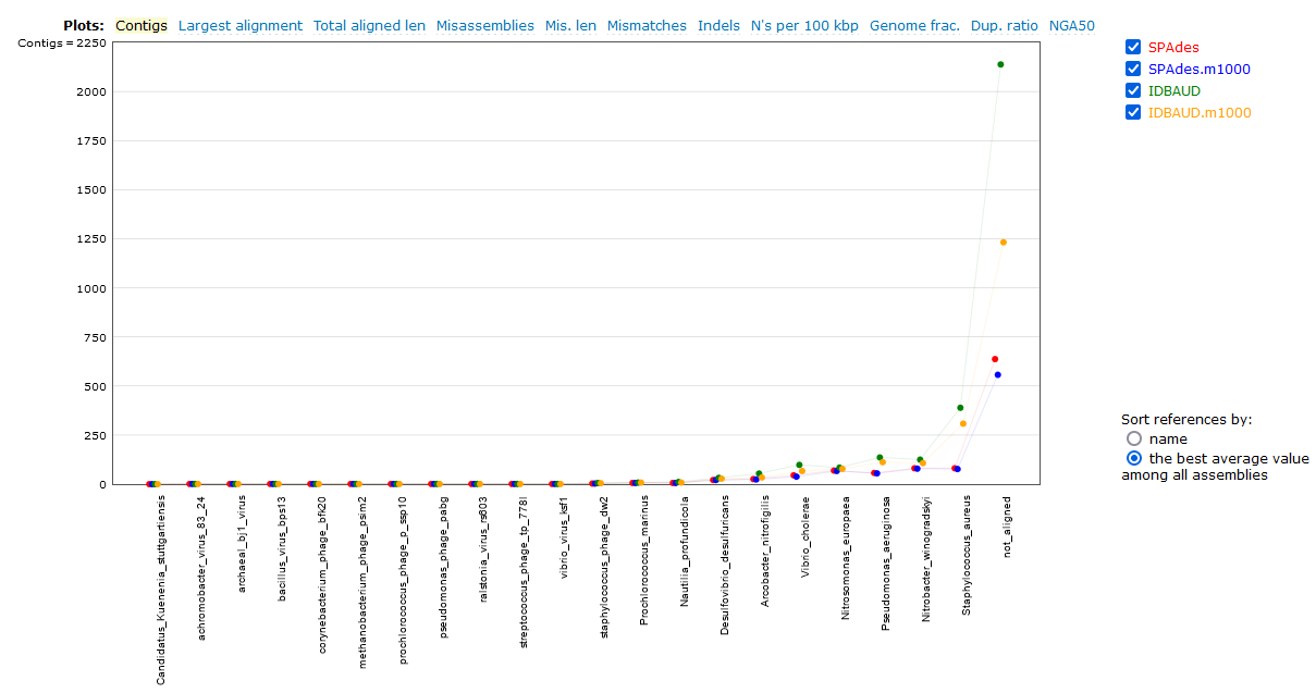
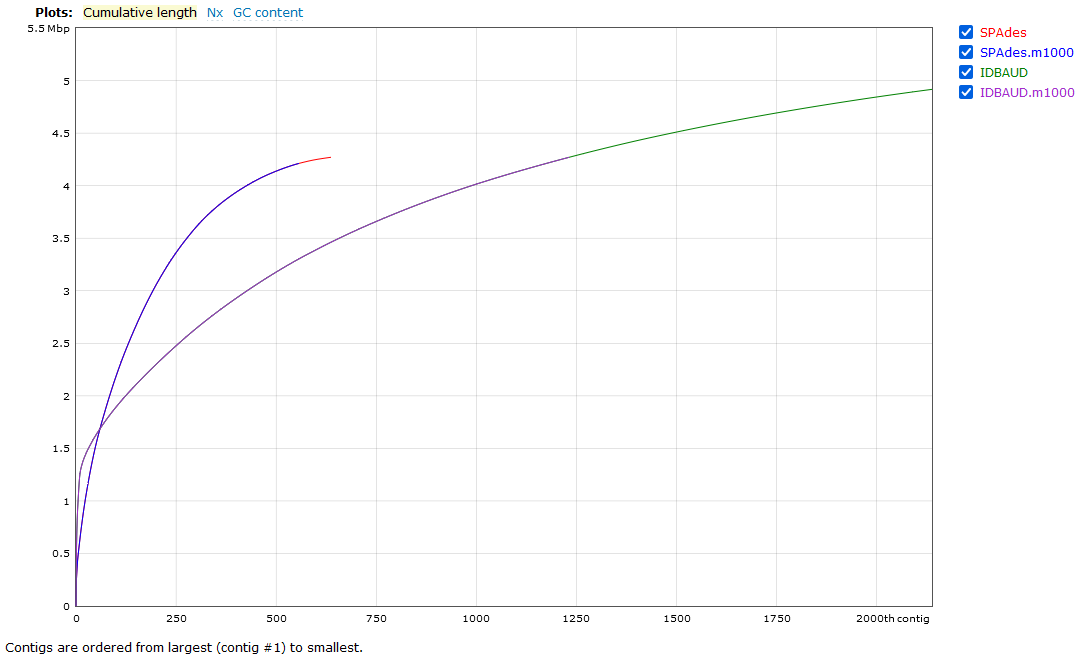
(Optional) Evaluating assemblies using MetaQUAST
For more genome-informed evaluation of the assembly, we can use the MetaQUAST tool to view our assembled metagenome. This is something of an optional step because, like QUAST, MetaQUAST aligns your assembly against a set of reference genomes. Under normal circumstances we wouldn't know the composition of the metagenome that led to our assembly. In this instance determining the optimal reference genomes for a MetaQUAST evaluation is a bit of a problem. For your own work, the following tools could be used to generate taxonomic summaries of your metagenomes to inform your reference selection:
- CLARK (DNA based. k-mer classification)
- Kaiju (Protein based, BLAST classification)
- Centrifuge (DNA based, sequence alignment classification)
- MeTaxa2 or SingleM (DNA based, 16S rRNA recovery and classification)
- MetaPhlAn2 (DNA based, clade-specific marker gene classification)
A good summary and comparison of these tools (and more) was published by Ye et al..
However, since we do know the composition of the original communities used to build this mock metagenome, MetaQUAST will work very well for us today. In your 4.evaluation/ directory you will find a file called ref_genomes.txt. This file contains the names of the genomes used to build these mock metagenomes. We will provide these as the reference input for MetaQUAST.
Remember to update <YOUR FOLDER> to your own folder
code
By now, you should be getting familiar enough with the console to understand what most of the parameters here refer to. The one parameter that needs explanation is the --max-ref-number flag, which we have set to 21. This caps the maximum number of reference genomes to be downloaded from NCBI which we do in the interest of speed. Since there are 21 taxa in the file ref_genomes.txt (10 prokaryote species and 11 viruses), MetaQUAST will download one reference genome for each. If we increase the --max-ref-number flag we will start to get multiple reference genomes per taxa provided which is usually desirable.
We will now look at a few interesting assembly comparisons.
Viewing HTML in Jupyter Hub
The NeSI Jupyter hub does not currently support viewing HTML that require Javascript (even if the browser you are running it in does). To view a basic version of the report, download the report file by navigating to the 4.evaluation/ directory, right-click metaquast_results.tar.gz and select download. You will need to decompress and extract the archive on your computer. Navigate to the folder with the extracted contents to open the report.html.