Gene synteny

Objectives

• Build a sulfur assimilation gene alignment figure to investigate gene synteny using R

---

Build a sulfur assimilation gene alignment figure to investigate gene synteny using R

When investigating the evolution of genomes, we sometimes want to consider not only the presence/absence of genes in a genome, but also how they are arranged (e.g. in an operon). For this exercise, we are going to visualise several sulfur assimilation genes from our MAGs and compare their arrangements.

This exercise involves the use of commands in bash and R. Before starting, make sure you have an active terminal, then navigate to the directory 11.data_presentation/gene_synteny/. Here, you'll find a copy of the annotations that came from DRAM (dram_annotations.tsv) and a directory of dereplicated bins in dastool_bins/.

1. Obtain contigs containing genes of interest (R)

In an open RStudio session, set your working directory to 11.data_presentation/gene_synteny/ and then load the required libraries and annotation file.

code

# Working directory
setwd("/nesi/nobackup/nesi02659/MGSS_U/<YOUR FOLDER>/11.data_presentation/gene_synteny/")

# Tidyverse packages
library(dplyr)
library(readr)
library(purrr)
library(stringr)
library(tidyr)

# Gene synteny
library(genoPlotR)

# KEGG API
library(KEGGREST)

# Import annotations
dram <- read_tsv("dram_annotations.tsv")

In order to be able to assimilate sulfate, prokaryotic genomes need to encode for the following KEGG orthologies which encode for an ATP-dependent thiosulfate/sulfate uptake system:

• K02045 (cysA)
• K02046 (cysU)
• K02047 (cysW)
• K02048 (cysP) or K23163 (sbp)

We'll subset the annotation file to obtain relevant rows and columns. In addtion to the bin and KO information, we require the gene position relative to the contig, strandedness, and the start and end position of the gene.

code

genes_of_interest <- c("K02048", "K23163", "K02046", "K02047", "K02045")

sulfate_assimilation <- dram %>%
  filter(ko_id %in% genes_of_interest) %>%
  select(fasta, scaffold, gene_position, ko_id, strandedness, start_position, end_position)

2. Check contiguity of genes

We need to check that the genes are contiguous (all on the same contig) and sequential. If there gaps between genes, we will need to fill them.

code

sulfate_assimilation %>%
  group_by(fasta) %>%
  distinct(scaffold) %>%
  tally(name = "n_contigs")

Console output

# A tibble: 4 × 2
  fasta n_contigs
  <chr>     <int>
1 bin_5         1
2 bin_7         2
3 bin_8         1
4 bin_9         1

We find that bin_7 is discontiguous. We need to identify how the genes of interest are distributed across the 2 contigs.

code

sulfate_assimilation %>%
  group_by(fasta, scaffold) %>%
  tally(name = "n_genes")

Console output

# A tibble: 5 × 3
# Groups:   fasta [4]
  fasta scaffold                                 n_genes
  <chr> <chr>                                      <int>
1 bin_5 bin_5_NODE_55_length_158395_cov_1.135272       4
2 bin_7 bin_7_NODE_54_length_158668_cov_0.373555       1
3 bin_7 bin_7_NODE_96_length_91726_cov_0.379302        4
4 bin_8 bin_8_NODE_12_length_355954_cov_0.516970       3
5 bin_9 bin_9_NODE_62_length_149231_cov_0.651774       4

Let's also check which gene is not contiguous.

code

sulfate_assimilation %>%
  filter(fasta == "bin_7") %>%
  select(scaffold, gene_position, ko_id)

Console output

# A tibble: 5 × 3
  scaffold                                 gene_position ko_id 
  <chr>                                            <dbl> <chr> 
1 bin_7_NODE_54_length_158668_cov_0.373555           136 K02048
2 bin_7_NODE_96_length_91726_cov_0.379302             18 K02045
3 bin_7_NODE_96_length_91726_cov_0.379302             19 K02047
4 bin_7_NODE_96_length_91726_cov_0.379302             20 K02046
5 bin_7_NODE_96_length_91726_cov_0.379302             21 K23163

Looks like there is a an operon that consists of sbp and cysAUW, then a discontiguous cysP.

We also need to check for gaps between genes of interest.

code

select(sulfate_assimilation, scaffold, gene_position)

Console output

# A tibble: 16 × 2
   scaffold                                 gene_position
   <chr>                                            <dbl>
 1 bin_5_NODE_55_length_158395_cov_1.135272           128
 2 bin_5_NODE_55_length_158395_cov_1.135272           132
 3 bin_5_NODE_55_length_158395_cov_1.135272           133
 4 bin_5_NODE_55_length_158395_cov_1.135272           134
 5 bin_7_NODE_54_length_158668_cov_0.373555           136
 6 bin_7_NODE_96_length_91726_cov_0.379302             18
 7 bin_7_NODE_96_length_91726_cov_0.379302             19
 8 bin_7_NODE_96_length_91726_cov_0.379302             20
 9 bin_7_NODE_96_length_91726_cov_0.379302             21
10 bin_8_NODE_12_length_355954_cov_0.516970           148
11 bin_8_NODE_12_length_355954_cov_0.516970           149
12 bin_8_NODE_12_length_355954_cov_0.516970           150
13 bin_9_NODE_62_length_149231_cov_0.651774            55
14 bin_9_NODE_62_length_149231_cov_0.651774            56
15 bin_9_NODE_62_length_149231_cov_0.651774            57
16 bin_9_NODE_62_length_149231_cov_0.651774            58

Here, we can see there is a gap in bin_5 where we need to fill 3 genes.

3. Subset relevant genes and positions

Based on the explorations above, we need to:

• Add genes 129-131 for scaffold bin_5_NODE_55_length_158395_cov_1.135272
• Remove bin_7_NODE_54_length_158668_cov_0.373555

code

# Add genes to bridge genes of interest for bin_5
bin_5_additions <- dram %>%
  filter(scaffold == "bin_5_NODE_55_length_158395_cov_1.135272" & gene_position %in% 129:131) %>%
  select(fasta, scaffold, gene_position, ko_id, strandedness, start_position, end_position)

# Remove extra scaffold from bin_7
sulfate_assimilation <- sulfate_assimilation %>%
  group_by(scaffold) %>%
  # Our discontiguous scaffold only has one entry
  filter(n() > 1)

# Combine both tables
sulfate_assimilation_coords <- bind_rows(sulfate_assimilation, bin_5_additions) %>%
  arrange(scaffold, gene_position) %>%
  mutate(gene_id = paste0(scaffold, "_", gene_position))

We will write out the results for processing in bash.

code

walk(
  unique(sulfate_assimilation_coords$fasta),
  function(bin) {
    write_tsv(
      filter(sulfate_assimilation_coords, fasta == bin),
      paste0(bin, ".goi.tsv")
    )
  }
)

4. Subset relevant scaffolds from bin sequences

Now, we need to return to the terminal.

Check that you're in 11.data_presentation/gene_synteny/

We'll use the previously generated table information to extract the scaffolds (using seqtk) we need from bin files.

code

module purge
module load seqtk/1.4-GCC-11.3.0

for i in *.goi.tsv; do
  bin=$(basename ${i} .goi.tsv)
  cut -f 2 ${i} | sed '1d' > tmp.scaffolds
  seqtk subseq dastool_bins/${bin}.fna tmp.scaffolds > ${bin}.goi.fna
done

5. Compare scaffolds using tBLASTx

With our scaffolds ready, we can now perform pairwise comparisons between them. You can choose to generate complete combinations for comparisons. Here, we will only compare between bins sequentially. As we are using the -subject flag, the comparisons are single-threaded (we cannot change this).

code

module purge
module load BLAST/2.16.0-GCC-12.3.0

bin_array=($(ls *.goi.fna | sed -e 's/.goi.fna//g'))

i=0
max_i=$(( ${#bin_array[@]}-1 ))

while [ $i -lt $max_i ]; do
  qbin=${bin_array[$i]} # Current bin as query
  sbin=${bin_array[$(($i+1))]} # Next bin as subject 

  printf "Comparing %s against %s\n" ${qbin} ${sbin}

  tblastx -query ${qbin}.goi.fna \
          -subject ${sbin}.goi.fna \
          -out blast_${qbin}_${sbin}.txt \
          -outfmt "7 std ppos frames"

  ((i++)) # Increment i after each comparison
done

-outfmt 7

You may be familiar with BLAST output format 6 as the tabular output from BLAST. Here, format 7 is the one with a commented header lines. This allows genoPlotR downstream to parse the columns appropriately. The proceeding arguments specifies a standard output std with additional columns for percentage of positive matches ppos and the translated frames for query/subject frames.

Now we have all the necessary files. We will return to the RStudio session for plotting.

6. Plot gene synteny

We first need to import all the relevant per bin files.

code

# Gene coordinates
goi_files <- list.files(pattern = ".*.goi.tsv")
goi <- map(goi_files, function(x) read_tsv(x)) %>%
  setNames(nm = str_remove(goi_files, "\\..*"))

# BLAST results
blast_files <- list.files(pattern = "blast.*")
blast <- map(blast_files, function(x) {
  read_comparison_from_blast(x)
}) %>%
  setNames(nm = str_remove(blast_files, ".txt"))

We will also create a data frame that has relevant information about the gene. In this case, we are using the gene symbol.

code

ko <- unique(bind_rows(goi)$ko_id)
kegg_records <- keggGet(ko[!is.na(ko)])
ko_annot <- map(kegg_records, function(entry) {
    data.frame("ko_id" = entry[["ENTRY"]], 
               "gene_symbol" = entry[["SYMBOL"]])
  }) %>%
  bind_rows()

We then create tracks of DNA segments and annotations that can be parsed by genoPlotR.

code

# DNA segments
ds_list <- map(goi, function(x) {
  coords <- x %>%
    select(gene_id, start_position, end_position, strandedness)
  colnames(coords) <- c("name", "start", "end", "strand")
  dna_seg(coords)
})

# Annotations that include gene symbols
annot_list <- map(goi, function(x) {
  data <- left_join(x, ko_annot, by = "ko_id") %>%
    select(gene_id, start_position, end_position, strandedness, ko_id, gene_symbol)
  annotation(
    x1 = data$start_position,
    x2 = data$end_position,
    text = ifelse(is.na(data$gene_symbol), "", data$gene_symbol)
  )
})

Finally, we can plot!

code

plot_gene_map(
  dna_segs = ds_list,
  comparisons = blast,
  annotations = annot_list,
  dna_seg_labels = names(ds_list),
  dna_seg_scale = TRUE,
  gene_type = "arrows"
)

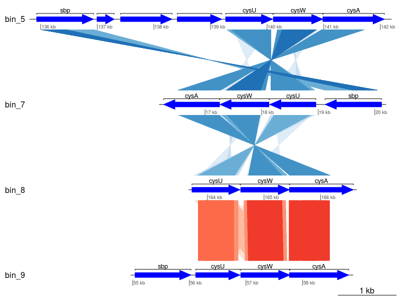
Seems a little messy, let's clean it up a little by only keeping those with the best matches (i.e., minimum E-value).

code

filt_blast <- map(blast, function(x) {
  group_by(x, name1, name2) %>%
    filter(e_value == min(e_value)) %>%
    ungroup() %>%
    as.comparison()
})

# Re-plot
plot_gene_map(
  dna_segs = ds_list,
  comparisons = filt_blast,
  annotations = annot_list,
  dna_seg_labels = names(ds_list),
  dna_seg_scale = TRUE,
  gene_type = "arrows"
)

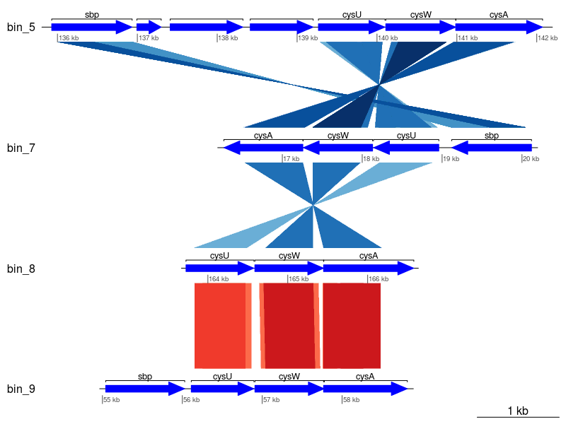
Much better! To further improve the plot, you might want to rearrange the tBLASTx comparisons and perhaps add additional information to the un-annotated genes based on hits to other databases (e.g., Pfam, TIGRFam, UniProt, etc.).