BayPass

The BayPass manual can be found here.

Citation

Gautier, M. (2015). Genome-wide scan for adaptive divergence and association with population-specific covariates. Genetics, 201(4), 1555-1579. https://doi.org/10.1534/genetics.115.181453

BayPass requires that the allele frequency data be on a population, not an individual basis. The genotyping data file is organized as a matrix with nsnp rows and 2 ∗ npop columns. The row field separator is a space. More precisely, each row corresponds to one marker, and the number of columns is twice the number of populations because each pair of numbers corresponds to each allele (or read counts for PoolSeq experiment) counts in one population.

To generate this population gene count data, we will work with the PLINK file. First, we have to fix the individual ID and population labels, as PLINK has pulled these directly from the VCF, which has no population information. We aim for population in column 1 and individual ID in column 2.

code

cd $DIR/data

awk '{print $2,"\t",$1}' $METADATA > starling_3populations_metadata_POPIND.txt

cd $DIR/analysis/baypass

PLINK=$DIR/data/starling_3populations.plink.ped

#remove first 2 columns
cut -f 3- $PLINK > x.delete

paste $DIR/data/starling_3populations_metadata_POPIND.txt x.delete > starling_3populations.plink.ped
rm x.delete 

cp $DIR/data/starling_3populations.plink.map .
cp $DIR/data/starling_3populations.plink.log .

Run the population-based allele frequency calculations.

code

module load PLINK/1.09b6.16 

plink --file starling_3populations.plink --allow-extra-chr --freq counts --family --out starling_3populations

Output

PLINK v1.90b6.16 64-bit (19 Feb 2020)          www.cog-genomics.org/plink/1.9/
(C) 2005-2020 Shaun Purcell, Christopher Chang   GNU General Public License v3
Logging to starling_3populations.log.
Options in effect:
  --allow-extra-chr
  --family
  --file starling_3populations.plink
  --freq counts
  --out starling_3populations

128824 MB RAM detected; reserving 64412 MB for main workspace.
.ped scan complete (for binary autoconversion).
Performing single-pass .bed write (5007 variants, 39 people).
--file: starling_3populations-temporary.bed +
starling_3populations-temporary.bim + starling_3populations-temporary.fam
written.
5007 variants loaded from .bim file.
39 people (0 males, 0 females, 39 ambiguous) loaded from .fam.
Ambiguous sex IDs written to starling_3populations.nosex .
--family: 3 clusters defined.
Using 1 thread (no multithreaded calculations invoked).
Before main variant filters, 39 founders and 0 nonfounders present.
Calculating allele frequencies... done.
Total genotyping rate is 0.723331.
Note: --freq 'counts' modifier has no effect on cluster-stratified report.
--freq: Cluster-stratified allele frequencies (founders only) written to
starling_3populations.frq.strat .

Manipulate file so it has BayPass format, numbers set for PLINK output file, and population number for column count.

code

tail -n +2 starling_3populations.frq.strat | awk '{ $9 = $8 - $7 } 1' | awk '{print $7,$9}' | tr "\n" " " | sed 's/ /\n/6; P; D' > starling_3populations_baypass.txt

Now we can run Baypass. It should run for about 5 minutes.

code

module purge
module load BayPass/2.31-intel-2022a

cd $DIR/analysis/baypass

i_baypass -npop 3 -gfile ./starling_3populations_baypass.txt -outprefix starling_3populations_baypass -nthreads 2

Run in R to make the anapod data. First, let us quickly download the utilities we need.

code

cd $DIR/programs
git clone https://github.com/andbeck/BayPass.git

Now let us generate some simulated data based on the parameters calculated from our genetic data.

code

module load R-bundle-Bioconductor/3.15-gimkl-2022a-R-4.2.1
R

code

library("ape")
setwd("~/outlier_analysis/analysis/baypass")
source("../../programs/BayPass/baypass_utils.R")

omega <- as.matrix(read.table("starling_3populations_baypass_mat_omega.out"))
pi.beta.coef <- read.table("starling_3populations_baypass_summary_beta_params.out", header = TRUE)
bta14.data <- geno2YN("starling_3populations_baypass.txt")
simu.bta <- simulate.baypass(omega.mat = omega, nsnp = 5000, sample.size = bta14.data$NN, beta.pi = pi.beta.coef$Mean, pi.maf = 0, suffix = "btapods")

q()

We now have the simulated genetic data. We can find the XtX statistic threshold above which we will consider genetic sites an outlier.

code

module purge
module load BayPass/2.31-intel-2022a

cd $DIR/analysis/baypass

i_baypass -npop 3 -gfile G.btapods -outprefix G.btapods -nthreads 2

XtX calibration; get the pod XtX threshold.

code

module load R-bundle-Bioconductor/3.15-gimkl-2022a-R-4.2.1
R

code

setwd("~/outlier_analysis/analysis/baypass")
source("~/outlier_analysis/programs/BayPass/baypass_utils.R")
library("ape")
library("corrplot")

pod.xtx <- read.table("G.btapods_summary_pi_xtx.out", header = T)

We compute the 1% threshold for the simulated neutral data.

code

pod.thresh <- quantile(pod.xtx$M_XtX ,probs = 0.99)
pod.thresh

q()

Output

     99% 
6.365673 

Your values may be slightly different as the simulated data will not be identical.

Next, we filter the data for the outlier SNPs by identifying those above the threshold.

code

cat starling_3populations_baypass_summary_pi_xtx.out | awk '$4>6.258372' > baypass_outliers.txt

SNP IDs are lost in BayeScan, line numbers are used as signifiers. We have previously created a list of SNPs in VCF and line numbers, which can be found at $DIR/analysis/starling_3populations_SNPs.txt which we will now reuse to generate a list of the outlier SNPS.

code

awk 'FNR==NR{a[$1];next} (($4) in a)' baypass_outliers.txt $DIR/analysis/starling_3populations_SNPs.txt | cut -f3 > baypass_outlierSNPIDs.txt
wc -l baypass_outlierSNPIDs.txt

Output

39 baypass_outlierSNPIDs.txt

Now let's find SNPs that are statistically associated with wingspan. To do this, we have to go back to the metadata and compute the average wingspan of each of our populations and place them in a file.

code

module load R-bundle-Bioconductor/3.15-gimkl-2022a-R-4.2.1
R

code

setwd("~/outlier_analysis/analysis/baypass")
metadata <- read.table("../../data/starling_3populations_metadata.txt", sep = "\t", header = FALSE)
str(metadata)
pop_metadata <- aggregate(V3 ~ V2, data = metadata, mean)
# Check mean wingspan
pop_metadata[, 2]
write(pop_metadata[, 2], "pop_mean_wingspan.txt")

q()

Output:

[1] 14.89805 19.63306 22.09655

Now we can run the third and final BayPass job, which will let us know which SNPs are statistically associated with wingspan.

code

module purge
module load BayPass/2.31-intel-2022a

cd $DIR/analysis/baypass

i_baypass -npop 3 -gfile starling_3populations_baypass.txt -efile pop_mean_wingspan.txt -scalecov -auxmodel -nthreads 2 -omegafile starling_3populations_baypass_mat_omega.out -outprefix starling_3populations_baypass_wing

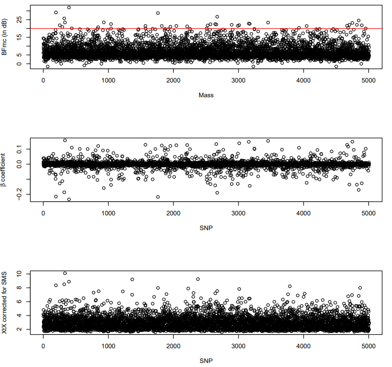
Next we plot the outliers. We are choosing a BF threshold of 20 dB, which indicates "Strong evidence for alternative hypothesis."

code

module load R-bundle-Bioconductor/3.15-gimkl-2022a-R-4.2.1
R

code

library(ggplot2)

setwd("~/outlier_analysis/analysis/baypass")

covaux.snp.res.mass <- read.table("starling_3populations_baypass_wing_summary_betai.out", header = T)
covaux.snp.xtx.mass <- read.table("starling_3populations_baypass_summary_pi_xtx.out", header = T)

pdf("Baypass_plots.pdf")
layout(matrix(1:3,3,1))
plot(covaux.snp.res.mass$BF.dB.,xlab="Mass",ylab="BFmc (in dB)")
abline(h=20, col="red")
plot(covaux.snp.res.mass$M_Beta,xlab="SNP",ylab=expression(beta~"coefficient"))
plot(covaux.snp.xtx.mass$M_XtX, xlab="SNP",ylab="XtX corrected for SMS")
dev.off()

Finally, let's generate the list of phenotype-associated SNP IDs.

code

cat starling_3populations_baypass_wing_summary_betai.out | awk '$6>20' > starling_3populations_baypass_wing_BF20.txt

wc -l starling_3populations_baypass_wing_BF20.txt

Output

45 starling_3populations_baypass_wing_BF20.txt

Filter the data sets for SNPS above BFmc threshold. These are out outlier SNPs that are associated with wingspan.

code

awk 'FNR==NR{a[$2];next} (($4) in a)' starling_3populations_baypass_wing_BF20.txt starling_3populations_SNPs.txt | cut -f3 > baypass_wingspan_outlierSNPIDs.txt

comm -12 <(sort baypass_wingspan_outlierSNPIDs.txt) <(sort baypass_outlierSNPIDs.txt) > double_outliers.txt

wc -l double_outliers.txt

Output

21 double_outliers.txt