PCAdapt
PCAdapt uses an ordination approach to find sites in a data set that are outliers with respect to background population structure. The PCAdapt manual is available here.
Citation
Privé, F., Luu, K., Vilhjálmsson, B. J., & Blum, M. G. B. (2020). Performing Highly Efficient Genome Scans for Local Adaptation with R Package pcadapt Version 4. Mol Biol Evol, 37(7), 2153-2154. https://doi.org/10.1093/molbev/msaa053
First, let's install PCAdapt and set your working directory.
Now let's load in the data - PCAdapt uses bed file types.
code
Produce K plot.
code

A K value of 3 is most appropriate, as this is the value of K after which the curve starts to flatten out more.
code
Output
                Length  Class  Mode
scores            117  -none-  numeric
singular.values     3  -none-  numeric
loadings        15021  -none-  numeric
zscores         15021  -none-  numeric
af               5007  -none-  numeric
maf              5007  -none-  numeric
chi2.stat        5007  -none-  numeric
stat             5007  -none-  numeric
gif                 1  -none-  numeric
pvalues          5007  -none-  numeric
pass             4610  -none-  numeric
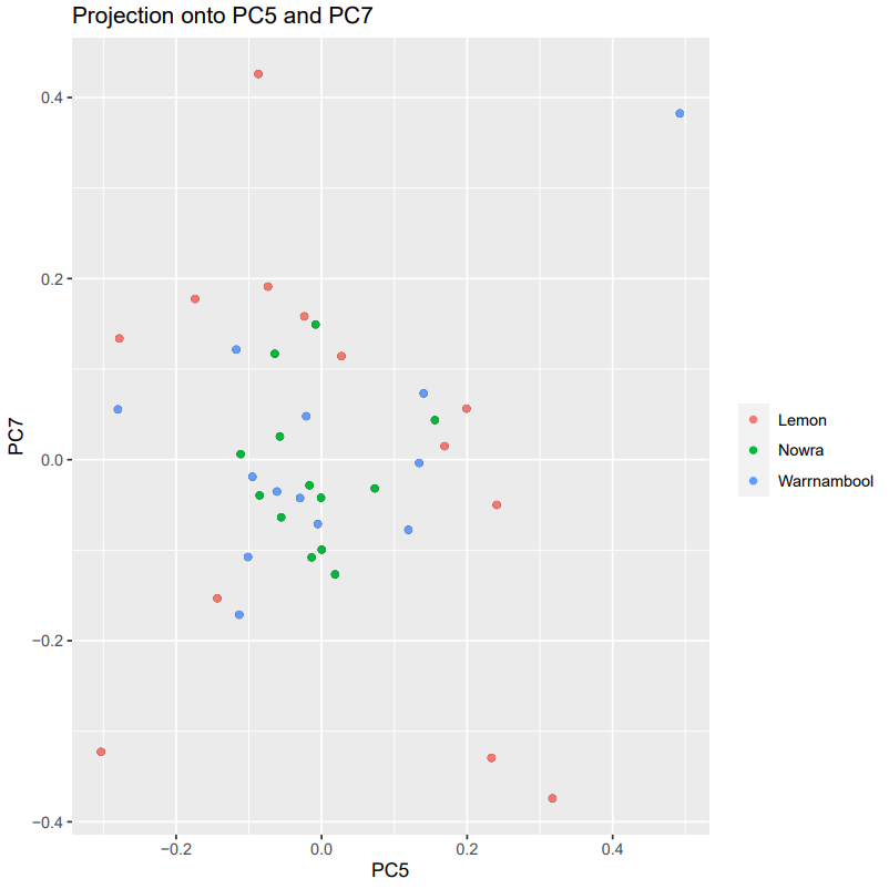
Investigate axis projections.
code
poplist.names <- c(rep("Lemon", 13),rep("Warrnambool", 13),rep("Nowra", 13))
print(poplist.names)

pdf("pcadapt_starlings_projection1v2.pdf")
plot(starlings_pcadapt_kplot, option = "scores", i = 1, j = 2, pop = poplist.names)
dev.off()

pdf("pcadapt_starlings_projection5v7.pdf")
plot(starlings_pcadapt_kplot, option = "scores", i = 5, j = 7, pop = poplist.names)
dev.off()

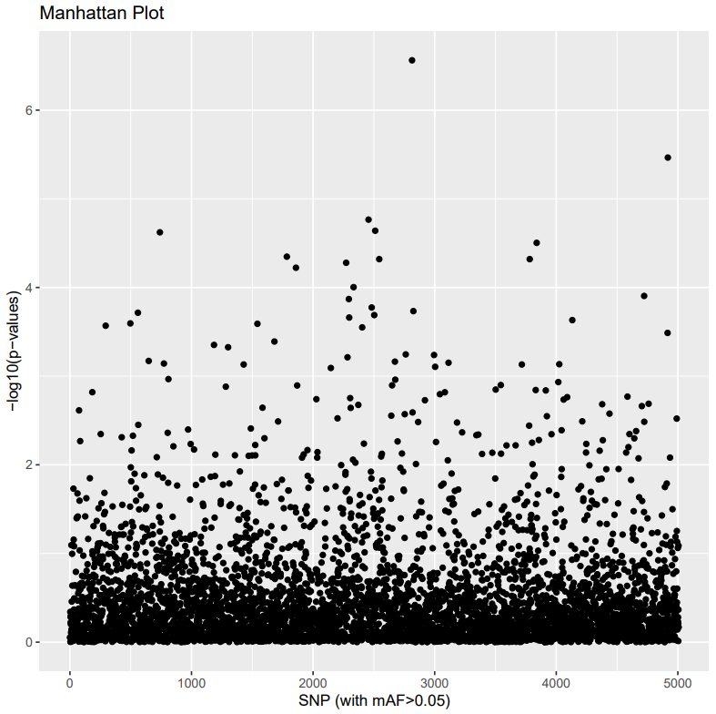
Investigate Manhattan and Q-Qplot.
Manhattan plots
This is a way to visualize the GWAS (genome-wide association study) p-values (or other statistical values) at each SNP locus along the genome.
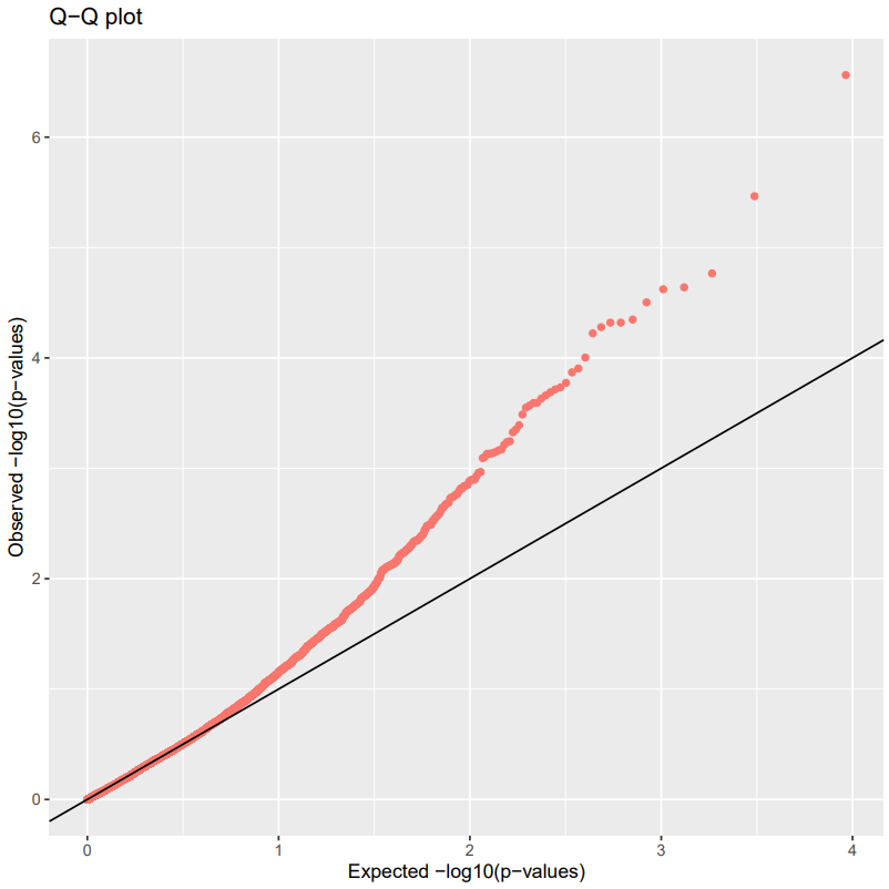
Q-Qplots
This is a quick way to check if your residuals are normally distributed. Check out more information here.
code
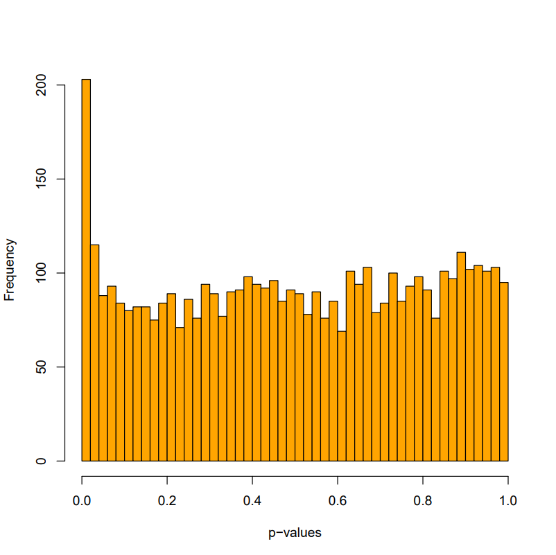
Plot and adjust the p-values.
code
code
After this, we will jump out of R and back into the command line by using the following command:
Mapping Outliers: PCAdapt
Find the SNP ID of the outlier variants.
The first thing we will do is create a list of SNPs in VCF and then assign line numbers that can be used to find matching line numbers in outliers (SNP IDs are lost in PCadapt & Bayescan, line numbers are used as signifiers).
We create this in the analysis/ directory because we will use it for more than just mapping the outlier SNPs for PCAdapt, we will also need it on day 2 for BayeScan and BayPass.
code
Now let us jump back into the pcadapt/ directory to continue working with our outliers. We select column 2 of the outlier file using the AWK command, which contains the number of outliers.
code
Make a list of outlier SNPS IDs.