VCFtools Windowed Fst
The VCFTools manual is available here.
Citation
Danecek, P., Auton, A., Abecasis, G., Albers, C. A., Banks, E., DePristo, M. A., Handsaker, R. E., Lunter, G., Marth, G. T., Sherry, S. T., McVean, G., Durbin, R., & Genomes Project Analysis, G. (2011). The variant call format and VCFtools. Bioinformatics, 27(15), 2156-2158. https://doi.org/10.1093/bioinformatics/btr330
Fst outliers help us to identify SNPs that behave abnormally in pairwise comparisons between populations.
We first need to use our metadata file (currently defined by the environmental variable METADATA) to make three individual files containing only the list of individuals in each population. We can do this by subsetting our sample metadata file, using the grep command to select lines that match each population's name, and then using awk to keep only the first column of metadata, i.e., the sample names.
code
# Load modules
module purge
module load VCFtools/0.1.15-GCC-9.2.0-Perl-5.30.1

# Enter data directory
cd $DIR/data

# Subset metadata
grep "Lemon" $METADATA | awk '{print $1}' > individuals_Lemon.txt
grep "War" $METADATA | awk '{print $1}' > individuals_War.txt
grep "Nowra" $METADATA | awk '{print $1}' > individuals_Nowra.txt
Now we can pick two populations to compare. Let's work with Lemon (short for Lemon Tree, QLD, AU) and War (short for Warnambool, VIC, AU) and perform an SNP-based Fst comparison.
code
cd $DIR/analysis/vcftools_fst

vcftools --vcf $VCF --weir-fst-pop $DIR/data/individuals_Lemon.txt --weir-fst-pop $DIR/data/individuals_War.txt --out lemon_war

head -n 5 lemon_war.weir.fst
Output
VCFtools - 0.1.15
(C) Adam Auton and Anthony Marcketta 2009

Parameters as interpreted:
        --vcf /nesi/nobackup/nesi02659/outlier_analysis_workshop/data/starling_3populations.recode.vcf
        --weir-fst-pop /nesi/nobackup/nesi02659/outlier_analysis_workshop/data/individuals_Lemon.txt
        --weir-fst-pop /nesi/nobackup/nesi02659/outlier_analysis_workshop/data/individuals_War.txt
        --keep /nesi/nobackup/nesi02659/outlier_analysis_workshop/data/individuals_Lemon.txt
        --keep /nesi/nobackup/nesi02659/outlier_analysis_workshop/data/individuals_War.txt
        --out lemon_war

Keeping individuals in 'keep' list
After filtering, kept 26 out of 39 Individuals
Outputting Weir and Cockerham Fst estimates.
Weir and Cockerham mean Fst estimate: 0.0067306
Weir and Cockerham weighted Fst estimate: 0.015
After filtering, kept 5007 out of a possible 5007 Sites
Run Time = 0.00 seconds
The important column is column 5: the Weighted Fst, from Weir and Cockerham’s 1984 publication.
Notice how there are as many lines as there are SNPs in the data set, plus one for a header. It is always a good idea to check your output to ensure everything looks as expected!
Next, instead of calculating pairwise population differentiation on an SNP-by-SNP basis, we will use a sliding window approach. The --fst-window-size 50000 refers to the window size of the genome (in base pairs) in which we are calculating one value: all SNPs within this window are used to calculate Fst. The --fst-window-step option indicates how many base pairs the window is moving down the genome before calculating Fst for the second window, then the third, and so on.
Sliding windows
These sliding windows only work on ordered SNPs on the same chromosome/scaffold/contig. If your data is not set up like this (i.e., all your SNPs are on a single pseudo-chromosome), then this method is not appropriate for your data, as it will make an assumption about where the SNPs are located with respect to one another.
code
vcftools --vcf $VCF --fst-window-size 50000 --fst-window-step 10000 --weir-fst-pop $DIR/data/individuals_Lemon.txt --weir-fst-pop $DIR/data/individuals_War.txt --out lemon_war

head -n 5 lemon_war.windowed.weir.fst
Output
VCFtools - 0.1.15
(C) Adam Auton and Anthony Marcketta 2009

Parameters as interpreted:
        --vcf /nesi/nobackup/nesi02659/outlier_analysis_workshop/data/starling_3populations.recode.vcf
        --fst-window-size 50000
        --fst-window-step 10000
        --weir-fst-pop /nesi/nobackup/nesi02659/outlier_analysis_workshop/data/individuals_Lemon.txt
        --weir-fst-pop /nesi/nobackup/nesi02659/outlier_analysis_workshop/data/individuals_War.txt
        --keep /nesi/nobackup/nesi02659/outlier_analysis_workshop/data/individuals_Lemon.txt
        --keep /nesi/nobackup/nesi02659/outlier_analysis_workshop/data/individuals_War.txt
        --out lemon_war

Keeping individuals in 'keep' list
After filtering, kept 26 out of 39 Individuals
Outputting Windowed Weir and Cockerham Fst estimates.
Weir and Cockerham mean Fst estimate: 0.0067306
Weir and Cockerham weighted Fst estimate: 0.015
After filtering, kept 5007 out of a possible 5007 Sites
Run Time = 1.00 seconds
Notice the output is different.
Notice the line count is different from the SNP-based Fst comparison; there are more lines in the sliding window-based Fst comparison. This is because there are more sliding windows across the chromosome in this data set than there are SNPs. Consider which of these steps is better for your data: the sliding window approach might not be the best in low-density SNP datasets.
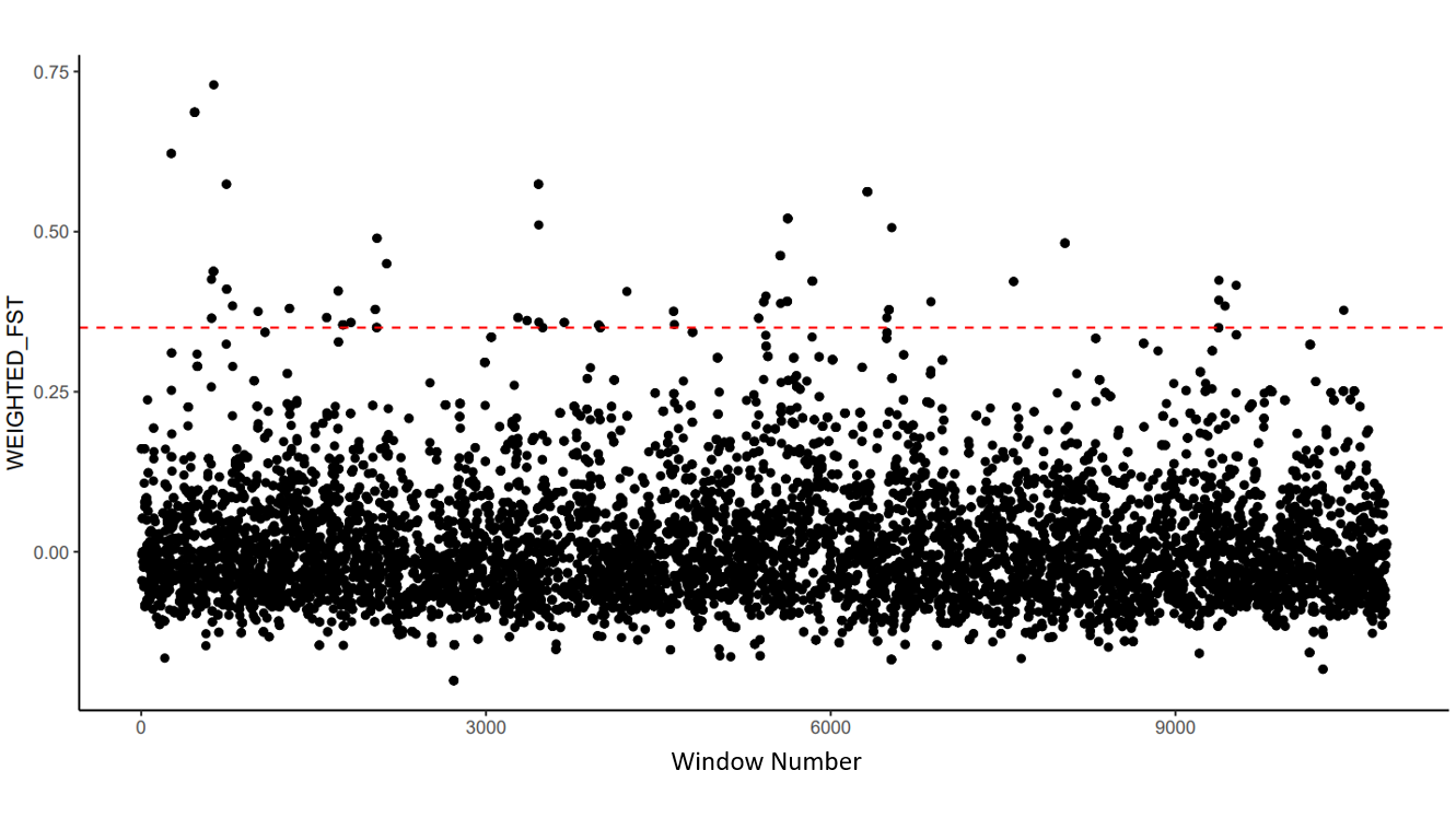
Now let us plot the Fst across the chromosome. To do this, we will add line numbers on our Fst file that will be used to order the Fst measurements across the x-axis of our Manhattan plot.
Note
X-axis values in the following plot are done using each outlier window's line number, as they are in order along the genome. Outlier windows are equally spaced, so line numbers are sufficient to capture the patterns along the genome. Consider that if you are plotting Fst values for SNPs (rather than windows), they may not be equally spaced along the genome, so SNP position may need to be used to make your Manhattan plots.
code
code
library("ggplot2")

setwd("~/outlier_analysis/analysis/vcftools_fst")

windowed_fst <- read.table("lemon_war.windowed.weir.fst.edit", sep="\t", header=TRUE)
str(windowed_fst)

quantile(windowed_fst$WEIGHTED_FST, probs = c(.95, .99, .999))
Output
'data.frame':   10837 obs. of  7 variables:
$ CHROM       : chr  "starling4" "starling4" "starling4" "starling4" ...
$ BIN_START   : int  60001 70001 80001 90001 100001 110001 120001 130001 140001 150001 ...
$ BIN_END     : int  110000 120000 130000 140000 150000 160000 170000 180000 190000 200000 ...
$ N_VARIANTS  : int  1 1 1 2 2 2 2 2 1 1 ...
$ WEIGHTED_FST: num  0.16089 0.16089 0.16089 -0.00374 -0.00374 ...
$ MEAN_FST    : num  0.1609 0.1609 0.1609 0.0402 0.0402 ...
$ X1          : int  2 3 4 5 6 7 8 9 10 11 ...
Choose the quantile threshold above which SNPs will be classified as outliers. In the code block below, we chose 99% (i.e., the top 1% of SNP windows).
code
Finally, we will generate a list of outlier SNP IDs. We do this by selecting all SNPs located in the outlier windows.
code
code
cut -f1-3 lemon_war.windowed.outliers > lemon_war.windowed.outliers.bed

vcftools --vcf $VCF --bed lemon_war.windowed.outliers.bed --out fst_outliers --recode

grep -v "^#" fst_outliers.recode.vcf | awk '{print $3}' > vcftoolsfst_outlierSNPIDs.txt

wc -l vcftoolsfst_outlierSNPIDs.txt
Output
VCFtools - 0.1.15
(C) Adam Auton and Anthony Marcketta 2009

Parameters as interpreted:
        --vcf /nesi/nobackup/nesi02659/outlier_analysis_workshop/data/starling_3populations.recode.vcf
        --out fst_outliers
        --recode
        --bed lemon_war.windowed.outliers.bed

After filtering, kept 39 out of 39 Individuals
Outputting VCF file...
        Read 107 BED file entries.
After filtering, kept 61 out of a possible 5007 Sites
Run Time = 0.00 seconds
We have a total of 61 outlier SNPs located across 107 outlier SNP windows.