7. Phased Assemblies in Action
What can you do with a phased assembly that you cannot do with a squashed assembly? Why does having a highly-continuous and highly-accurate assembly matter? In same cases, you don’t need an assembly like that, e.g., if doing targeted sequencing of a region of interest that fits inside the length of a read. Conversely, some applications require a good assembly, e.g., when studying repetitive DNA, especially long and/or interspersed repeats. Phasing is also helpful when the haplotypes differ, especially when those differences are structural in nature (e.g., copy number variants or large insertions, deletions, duplications, or inversions). Let’s take a look at the repeats in chromosome Y of our HG002 assembly.
Visualizing Repeats using ModDotPlot
ModDotPlot is a tool for visualizing tandem repeats using dot plots, similar to StainedGlass (Vollger et al. 2022), but using sketching methods to radically reduce the computational requirements. Visualizing tandem repeats like this requires an assembly that spans all the repeat arrays and assembles them accurately, making this a potent example of the benefits of combining highly-accurate, long reads (like PacBio HiFi) with ultralong reads from ONT in the assembly process with hifiasm (Cheng et al. 2022) or Verkko (Rautiainen et al. 2023). Take a moment, and consider that. You can’t do this with reads alone (even long reads). Mapping to a good reference (e.g., CHM13-T2T) for your species of interest (if one exists) won’t work either because the alignment software can’t distinguish between repeat copies.
What are sketching methods ?
Sketching is a technique to create reduced-representations of a sequence. The most widely-known option for sketching is probably minimizers, made particularly popular with tools like minimap2 (Li 2018), which applies minimizers to the alignment problem. We discussed minimizers earlier when running MashMap. The minimizer for any given window is the lexicographically smallest canonical k-mer. Several variants to minimizers exist, e.g., syncmers, minmers, and modimizers, the latter of which is used in ModDotPlot. Each sketching method has different properties depending on how they select the subsequence used to represent a larger area, whether they allow overlaps, whether a certain density of representative sequences is enforced in any given window, whether the neighboring windows are dependent on eachother, etc. In general, the representative sequences are found by sliding along the sequence and selecting a representative subsequence in the given window.
Many other tools use sketching in some way, here are a few examples:
- Mash (Ondov et al. 2016)
- MashMap (Kille et al. 2023)
-
MBG (Rautiainen & Marschall 2021) <-- Used in Verkko (Rautiainen et al. 2023)!
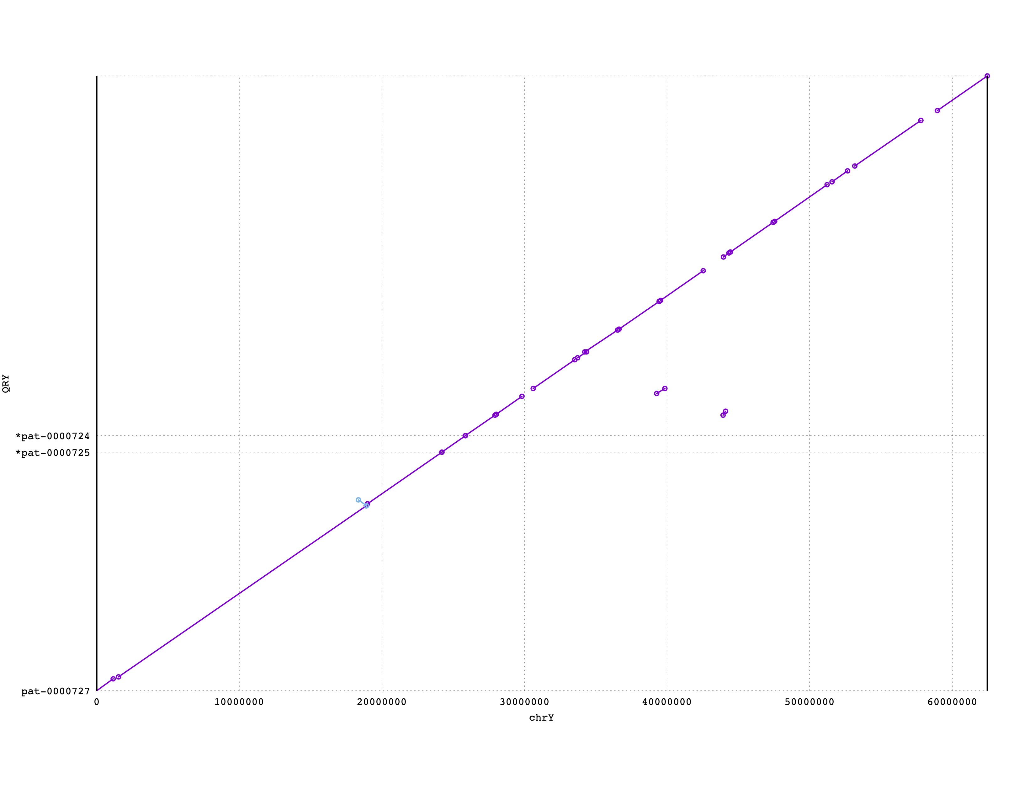
We're going to run ModDotPlot on part of the Y chromosome from our earlier assembly. First we’ll need to identify the appropriate chunk, which can be done a few different ways depending on the sequence you’re looking for. ChrY somtimes appears tied on only one end to chrX in the Bandage plot, making it easy to identify the Y node (which is shorter than the longer X node). This method may not get all of the Y chromosome because it may be in separate pieces (i.e., it isn’t T2T), and we often see chrX and chrY untangled from eachother in one or two pieces each, so topology of the graph isn’t always a reliable option (though, we recommend labelling the graph with the chromosome names to get a feel for how your assembly looks). The ideal way is to map some known sequence against your assembly or to map your assembly against a known reference. Since we’re using data from HG002 (a human), we can map against the human CHM13-T2T reference.
Initial setup
Make a directory to work in
Get the files
code
ln -s /nesi/nobackup/nesi02659/LRA/resources/chm13/chm13v2.0.fa chm13.fa
ln -s /nesi/nobackup/nesi02659/LRA/resources/assemblies/verkko/full/trio/assembly/assembly.haplotype2.fasta hg002.hap2.fa
ln -s /nesi/nobackup/nesi02659/LRA/resources/assemblies/verkko/full/trio/assembly/assembly.haplotype2.fasta.fai hg002.hap2.fa.fai
Note that we’re cheating a bit. We could map against the entire diploid assembly, but we’ve already determined that chrY is in haplotype2, so we’ll save some time and work with only that haplotype.
Find chrY contigs with MashMap
Do the alignments
We’ll do the alignments with MashMap (Kille et al. 2023). This should take ~25 minutes with 4 CPUs and should use <4 GB RAM. With 16 CPUs, it should take ~4 minutes and will use <8 GB RAM. This command is the same as the one you ran earlier, except that this time it is on haplotype2 and the percent identity threshold is lower, which should help us recruit alignments in the satellites on chrY. We’ll use pre-computed results to avoid needing to wait for the job to complete, but this is what the command would look like:
view, but do not run this code
How would I submit this as a job?
Submit it as a job with sbatch. First copy the command into a
script named mashmap.sh:
#!/bin/bash -e

#SBATCH --account       nesi02659
#SBATCH --job-name      mashmap
#SBATCH --cpus-per-task 16
#SBATCH --time          00:20:00
#SBATCH --mem           8G
#SBATCH --partition     milan
#SBATCH --output        slurmlogs/%x.%j.out
#SBATCH --error         slurmlogs/%x.%j.err


module purge
module load MashMap/3.0.4-Miniconda3

mashmap -f "one-to-one" \
    -k 16 --pi 90 \
    -s 100000 -t 16 \
    -r chm13.fa \
    -q hg002.hap2.fa \
    -o hg2hap2-x-chm13.ssv
Then submit the job with the following command:
Get the pre-computed results
code
View the output file
There is more information present than we need, and we can simplify things by looking at long alignments only.
Subset the alignments
code
What is the awk command doing ?
This awk command is keeping only alignments (remember, one
alignment is on each line of the file) that map to chrY; the sixth column
is the "reference" or "target" sequence name. The third and fourth columns
are respectively the start and stop positions of the aligned region on the
"query" sequence (i.e., a contig from our assembly); thus, we’re
keeping only alignments that are 1 Mbp or longer. This also has the
consequence of ignoring contigs that are shorter than 1 Mbp.
Wait, what are each of the columns again?
According to the MashMap README
The output is space-delimited with each line consisting of query name, length, 0-based start, end, strand, target name, length, start, end, and mapping nucleotide identity.
Re-written as a numbered list:
MashMap output columns
- query name
- length
- 0-based start
- end
- strand
- target name
- length
- start
- end
- mapping nucleotide identity
View the output file
Now that we’ve culled the alignments, viewing them should be much easier:
Which contigs belong to chrY?
Answer
pat-0000724, pat-0000725, and pat-0000727 are probably chrY.
Others may be as well, but it is difficult to tell without a more refined investigation, and this is sufficient for our purposes.
How can we tell?
Anything with a long, high-identity alignment is a pretty good candidate, especially if the contig was determined to be paternal using trio markers (as these were). One thing that may help is seeing what percentage of the contig is covered by each alignment:
code
To prevent you from having to do the math in your head, here are the
percentages of each contig aligned to chrY (sum of the final column in
the hg2hap2-x-chm13.gt1m-chrY.annotated.txt file):
| HG002 Contig | % aligned to chrY |
| pat-0000724 | 84.332% |
| pat-0000725 | 99.9999% |
| pat-0000727 | 98.342% |
More short contigs may also belong to chrY, but we would need to investigate more carefully to find them. We would want to confirm whether telomeres are present on the end of the terminal contigs. Also, we do not expect perfect or complete alignments here; not only are we using a sketching-based alignment method, but any aligner would likely struggle when aligning repetitve DNA. So, how much of chrY did we capture with these three contigs? You can see that these three contigs cover the majority, if not all, of chrY:
Create self dot plots for each contig
ModDotPlot is still in development, and it cannot currently support doing multiple self comparisons at one time. We will need to create separate fasta files for our contigs of interest.
Create and index subset fastas
code
Run ModDotPlot
On sequences of this size, ModDotPlot is relatively quick. It has a reasonable
memory footprint for sequences <10 Mbp, but memory usage can exceed 20 GB for
large sequences (>100 Mbp). Let's create a script to submit with
sbatch. Paste the following into moddotplot.sh
code
#!/bin/bash -e

#SBATCH --account       nesi02659
#SBATCH --job-name      moddotplot
#SBATCH --cpus-per-task 4
#SBATCH --time          00:10:00
#SBATCH --mem           8G
#SBATCH --partition     milan
#SBATCH --output        slurmlogs/%x.%j.log

module purge
module load ModDotPlot/2023-06-gimkl-2022a-Python-3.11.3

for CTG in pat-000072{4,5,7}
do
    moddotplot \
        -k 21 -id 85 \
        -i hg002.hap2.${CTG}.fa \
        -o mdp_hg002-${CTG}
done
Then submit with sbatch:
What do these parameters do ?
You can run moddotplot -h to find out (and enjoy some excellent ASCII art).
Here are the options we used:
Required input:
  -i INPUT [INPUT ...], --input INPUT [INPUT ...]
                        Path to input fasta file(s)

Mod.Plot distance matrix commands:
  -k KMER, --kmer KMER  k-mer length. Must be < 32 (default: 21)

  -id IDENTITY, --identity IDENTITY
                        Identity cutoff threshold. (default: 80)

  -o OUTPUT, --output OUTPUT
                        Name for bed file and plots. Will be set to input fasta file name if not provided. (default: None)
Inspect the output files
First, take a look at the log file:
Then note that for every run, we created _HIST.png and _TRI.png files. The
HIST files show the distribution of the Percent Identity of the alignments. The
TRI files show everything above (or below, depending on how you look at it) the
diagonal of the dotplot, rotated such that the diagonal is along the X-axis of
the plot. Go ahead a view these files now.
What do you observe?