5. Assembly QC¶

Now that we have understood our data types (day 1) and put them through an assembly algorithm (day 2), we have this file of A's, T's, C's, and G's that's supposed to be our assembly. This file is meant to represent a biological reality, so let's try to assess its quality through several lens, some biological and some more technical. One way to remember the ways we evaluate assemblies is by thinking about the "3C's": contiguity, correctness, and completeness.

Food for thought

What do you think a 'good' de novo assembly looks like?
What are some qualities of an assembly that you might be interested in measuring?

Contiguity (assembly statistics using gfastats)¶

Recall that the sequences in our assembly are referred to as contigs.

Normally, when we receive a hodgepodge of things with different values of the same variable, such as our contigs of varying lengths, we are inclined to use descriptive statistics such as average or median to try to get a grasp on how our data looks. However, it can be hard to compare average contig length between assemblies—if they have the same total size and same number of contigs, it's still the same average, even if it's five contigs of 100bp, or one 460 bp contig and four 10bp ones! This matters for assembly because ideally we want fewer contigs that are larger.

Median comes closer to reaching what we're trying to measure, but it can be skewed by having many very small contigs, so instead a popular metric for assessing assemblies is N50.

The N50 is similar to the median in that one must first sort the numbers, but then instead of taking the middle value, the N50 value is the length of the first contig that is equal to or greater than half of the assembly sum. But that can be hard to understand verbally, so let's look at it visually:

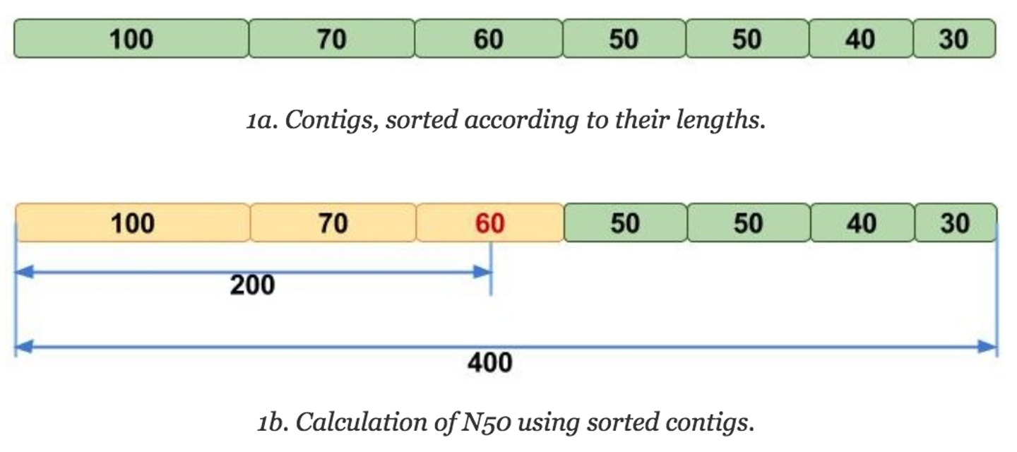Image adapted from Elin Videvall at The Molecular Ecologist.

The N50 can be interpreted as such: given an N50 value, 50% of the sequence in that assembly is contained in contigs of that length or longer. Thus, N50 has been traditionally used as the assembly statistic of choice for comparing assemblies, as it's more intuitive (compared to average contig length) to see that an assembly with an N50 value of 100Mbp is more contiguous than one with an N50 value of 50MBp, since it seems like there are more larger contigs in the former assembly.

Another statistic that is often reported with N50 is the L50, which is the rank of the contig that gives the N50 value. For instance, in the above image, the L50 would be 3, because it would be the third largest contig that gives the N50 value. L50 is useful for contextualizing the N50, because it gives an idea of how many contigs make up that half of your assembly.

N50 or NG50?

Another measurement you might see is NG50. This is the N50 value, just calculated using a given genome size instead of the sum of the contigs.

Given how the N50 value can be so affected by addition or removal of small contigs, another metric has come into use: the area under the (N50) curve, or the auN value. Though N50 is measured at the 50% mark, we could make similar values for any value of x, for instance N30 would be the value where 30% of the sequence in that assembly is of that length or longer. These metrics are thus called Nx statistics, and one could plot them against contig length to get an Nx curve, which gives a more nuanced view of the actual contig size distribution of your assembly.

Image adapted from Heng Li's blog, which in turn adapts it from a NIBS workshop

auN tries to capture the nature of this curve, instead of a value from an arbitrary point on it. On the above example, each step on the curve represents a contig (length on the y-axis), so the black curve is the most contiguous as it has one contig that covers over 40% of the assembly. Despite that, this assembly would have the same N50 value (on the x-axis) as multiple other assemblies that are more fragmented in the same area.

Run gfastats on a FASTA¶

Let's get some basic statistics for an assembly using a tool called gfastats, which will output metrics such as N50, auN, total size, etc. We can try it out on a Verkko trio assembly of HG002 that's already been downloaded onto NeSI.

code

## let's symlink the file in a way that's easier to refer to
cd ~/lra
mkdir -p day3_assembly_qc/gfastats
cd day3_assembly_qc/gfastats
ln -s /nesi/nobackup/nesi02659/LRA/resources/assemblies/verkko/full/trio/assembly/assembly.*.fasta .
ls -la          # you should see a bunch of "files" that are actually symlinks pointing to their actual content

Now we're ready to roll!

module purge
module load gfastats
gfastats assembly.haplotype1.fasta

Shouldn't take about 10 seconds

Output

+++Assembly summary+++: 
# scaffolds: 81
Total scaffold length: 3025610697
Average scaffold length: 37353218.48
Scaffold N50: 112270693
Scaffold auN: 120344050.34
Scaffold L50: 10
Largest scaffold: 242261106
Smallest scaffold: 7980
# contigs: 95
Total contig length: 3024505387
Average contig length: 31836898.81
Contig N50: 101137168
Contig auN: 98109753.40
Contig L50: 12
Largest contig: 201096255
Smallest contig: 7980
# gaps in scaffolds: 14
Total gap length in scaffolds: 1105310
Average gap length in scaffolds: 78950.71
Gap N50 in scaffolds: 222184
Gap auN in scaffolds: 267123.76
Gap L50 in scaffolds: 2
Largest gap in scaffolds: 425849
Smallest gap in scaffolds: 1000
Base composition (A:C:G:T): 893171444:618413603:615928136:896992204
GC content %: 40.81
# soft-masked bases: 0
# segments: 95
Total segment length: 3024505387
Average segment length: 31836898.81
# gaps: 14
# paths: 81

Run gfastats on a GFA¶

Remember that the file we initially got was an assembly graph—what if we wanted to know some graph-specific stats about our assembly, such as number of nodes or disconnected components? We can also assess that using gfastats.

code

ln -s /nesi/nobackup/nesi02659/LRA/resources/assemblies/verkko/full/trio/assembly/5-untip/unitig-normal-connected-tip.gfa .
gfastats --discover-paths unitig-normal-connected-tip.gfa

Output

+++Assembly summary+++: 
# scaffolds: 2312
Total scaffold length: 4179275425
Average scaffold length: 1807645.08
Scaffold N50: 10829035
Scaffold auN: 11407399.64
Scaffold L50: 134
Largest scaffold: 38686347
Smallest scaffold: 1987
# contigs: 2312
Total contig length: 4179275425
Average contig length: 1807645.08
Contig N50: 10829035
Contig auN: 11407399.64
Contig L50: 134
Largest contig: 38686347
Smallest contig: 1987
# gaps in scaffolds: 0
Total gap length in scaffolds: 0
Average gap length in scaffolds: 0.00
Gap N50 in scaffolds: 0
Gap auN in scaffolds: 0.00
Gap L50 in scaffolds: 0
Largest gap in scaffolds: 0
Smallest gap in scaffolds: 0
Base composition (A:C:G:T): 1180405407:909914907:908088683:1180866428
GC content %: 43.50
# soft-masked bases: 0
# segments: 2312
Total segment length: 4179275425
Average segment length: 1807645.08
# gaps: 0
# paths: 2312
# edges: 5790
Average degree: 2.50
# connected components: 47
Largest connected component length: 530557693
# dead ends: 562
# disconnected components: 184
Total length disconnected components: 60717682
# separated components: 231
# bubbles: 8
# circular segments: 11

What's the --discover-paths flag for?

gfastats tries to clearly distinguish contigs from segments, so it will not pick up on contigs in a GFA without paths defined. To get the contig stats as well as graph stats from these GFAs, you'll need to add the --discover-paths flag.

Check out the graph-specific statistics at the end of the output.

Compare two graphs' stats¶

Now that we know how to get the statistics for one assembly, let's get them for two so we can actually compare them. We already compared a Verkko HiFi-only and HiFi+ONT graph visually, so let's do it with assembly stats this time. We're going to use a one-liner to put the assembly stats side-by-side, because it can be kind of cumbersome to scroll up and down between two separate command line runs and their outputs.

code

paste \
<(gfastats -t --discover-paths /nesi/nobackup/nesi02659/LRA/resources/assemblies/verkko/full/trio/assembly/1-buildGraph/hifi-resolved.gfa) \
<(gfastats -t --discover-paths /nesi/nobackup/nesi02659/LRA/resources/assemblies/verkko/full/trio/assembly/5-untip/unitig-normal-connected-tip.gfa \
| cut -f 2)

paste is a command that pastes two files side by side
The <(COMMAND) syntax is called process substitution, and it passes the output of the command(s) inside the parentheses to another command (here it is passing the gfastats output to paste), and can be useful when using a pipe (|) might not be possible
The -t flag in gfastats specifies that the output should be tab-delimited, which makes it more computer-parsable
The cut command in the substitution is just getting the actual statistics column from the gfastats output, because the first column is the name of the statistic

Your output should look something like this:

Output

# contigs       68252   2312
Total contig length     3858601893      4179275425
Average contig length   56534.63        1807645.08
Contig N50      223090  10829035
Contig auN      638121.24       11407399.64
Contig L50      4232    134
Largest contig  23667669        38686347
Smallest contig 1608    1987
# gaps in scaffolds     0       0
Total gap length in scaffolds   0       0
Average gap length in scaffolds 0.00    0.00
Gap N50 in scaffolds    0       0
Gap auN in scaffolds    0.00    0.00
Gap L50 in scaffolds    0       0
Largest gap in scaffolds        0       0
Smallest gap in scaffolds       0       0
Base composition (A:C:G:T)      1089358958:840831652:838233402:1090177881       1180405407:909914907:908088683:1180866428
GC content %    43.51   43.50
# soft-masked bases     0       0
# segments      68252   2312
Total segment length    3858601893      4179275425
Average segment length  56534.63        1807645.08
# gaps  0       0
# paths 68252   2312
# edges 181274  5790
Average degree  2.66    2.50
# connected components  45      47
Largest connected component length      496518810       530557693
# dead ends     684     562
# disconnected components       18      184
Total length disconnected components    7267912 60717682
# separated components  63      231
# bubbles       4312    8
# circular segments     31      11

Output explained

... where the first column is the stats from the HiFi-only assembly graph, and the second column is the stats from the HiFi+ONT assembly graph. Notice how the HiFi-only graph has way more nodes than the HiFi+ONT one, like we'd seen in Bandage. Stats-wise, this results in the HiFi-only graph having a N50 value of 223 Kbp while the HiFi+ONT one is 10.8 Mbp, a whole order of magnitude larger. For the HiFi-only graph, though, there's a bigger difference between its N50 value and its auN value: 223 Kbp vs. 638 Kbp, while the HiFi+ONT stats have a smaller difference of 10.8 Mbp vs. 11.4 Mbp. This might be due to the HiFi-only graph having on average shorter segments and more of the shorter ones, since it doesn't have the ONT data to resolve the segments into larger ones.

Correctness (QV using Merqury)¶

Correctness refers to the base pair accuracy, and can be measured by comparing one's assembly to a gold standard reference genome. This approach is limited by 1) an assumption about the quality of the reference itself and the closeness between it and the assembly being compared, and 2) the need for a reference genome at all, which many species do not have (yet). To avoid this, we can use Merqury: a reference-free suite of tools for assessing assembly quality (particularly w.r.t. error rate) using k-mers and the read set that generated that assembly. If an assembly is made up from the same sequences that were in the sequencing reads, then we would not expect any sequences (k-mers) in the assembly that aren't present in the read set—but we do find those sometimes, and those are what Merqury flags as error k-mers. It uses the following formula to calculate QV value, which typically results in QVs of 50-60:

\[ \Large E=1-P=1-\left (1-\frac{K_{\textrm{asm}}}{K_{\textrm{total}}} \right ) ^{\frac{1}{k}} \]

OK, but what does 'QV' mean, anyway?

The QV that Merqury is interpreted similarly to the commonly used Phred quality scale, which might be familiar to those who have done short-read sequencing or are otherwise acquainted with FASTQ files. Phred quality scores are logarithmically related to error-probability, such that: - Phred score of 30 represents a 1 in 1,000 error probability (i.e., 99.9% accuracy) - Phred score of 40 represents a 1 in 10,000 error probability (i.e., 99.99% accuracy) - Phred score of 50 represents a 1 in 100,000 error probability (i.e., 99.999% accuracy) - Phred score of 60 represents a 1 in 1,000,000 error probability (i.e., 99.9999% accuracy)

Merqury operates using k-mer databases like the ones we generated using meryl, so that's what we'll do now.

Running Meryl and GenomeScope on the E. coli Verkko assembly¶

Let's try this out on the E. coli Verkko assembly. First we need a Meryl database, so let's generate that.

code

cd ~/lra
mkdir -p day3_assembly_qc/merqury
cd day3_assembly_qc/merqury

We just made a directory for our runs, now let's sym link the fasta and reads here so we can refer to them more easily

ln -s ../../day2_assembly/verkko_test/assembly/assembly.fasta .
ln -s ../../day2_assembly/verkko_test/hifi.fastq.gz .

Now we can run it!

module purge
module load Merqury
sbatch --account nesi02659 --job-name=meryl --time=00:15:00 --cpus-per-task 8 --mem=24G -p milan --wrap="meryl count k=30 memory=24 threads=8 hifi.fastq.gz output read-db.meryl"

--wrap ???

Previously, we used the sbatch command to submit a slurm script to the cluster and the slurm job handler. The sbatch command can actually take a lot of parameters like the ones we included in the beginning of our script, and one of those parameters is --wrap which kind of wraps whatever command you give it in a Slurm wrapper so that the cluster can schedule it as if it was a Slurm script.

Take note that running a process in this manner is not reproducible. Unless you have access to the history logs, other researchers are not able to know what parameters you have used. Therefore, it is advisable to write it out in a Slurm script as below:

code

#!/bin/bash -e
#SBATCH --account=nesi02659
#SBATCH --job-name=meryl
#SBATCH --time=00:15:00
#SBATCH --cpus-per-task=8
#SBATCH --mem=24G
#SBATCH --partition=milan

# Modules
module purge
module load Merqury/1.3-Miniconda3

# Run
meryl count k=30 memory=24 threads=8 \
  hifi.fastq.gz \
  output read-db.meryl

That shouldn't take too long to run. Now we have a Meryl DB for our HiFi reads. If we're curious about the distribution of our k-mers, we can use Meryl generate a histogram of the counts to show us how often a k-mer occurs only once in the reads, twice, etc.

How would you go about trying to do this with meryl?

When you want to use a tool to do something (and you are decently confident that the tool can actually do it), then a good point to start is just querying the tool's manual or help dialogue. Try out meryl --help and see if there's a function that looks like it could generate the histogram we want. ~~spoiler alert: it's meryl histogram read-db.meryl~~

If you tried to run that command with the output straight to standard out (i.e., your terminal screen), you'll see it's rather overwhelming and puts you all the way at the high, high coverage k-mer counts, which are only one occurrence. Let's look at just the first 100 lines instead.

code

meryl histogram read-db.meryl > read-db.hist
head -n 100 read-db.hist

This is more manageable, and you can even kind of see the histogram forming from the count values. There's a lot of k-mers that are present at only one copy (or otherwise very low copy) in the read set: these are usually sequencing errors, because there's a lot of these k-mers present at low copy. Because the sequence isn't actually real (i.e., it isn't actually in the genome and isn't actually serving as sequencing template), these k-mers stay at low copy. After these error k-mers, there's a dip in the histogram until about the 24–28 copy range. This peak is the coverage of the actual k-mers coming from the genome that you sequenced, thus it corresponds to having coverage of ~26X in this read set. We only have one peak here because this is a haploid dataset, but if your dataset is diploid then expect two peaks with the first peak varying in height depending on heterozygosity of your sample.

"What if I want a pretty graph instead of imagining it?" Good news—there's ~~an app~~ a program for that. GenomeScope is a straightforward program with an online web page where you can just drop in your meryl histogram file and it will draw the histogram for you as well as use the GenomeScope model to predict some genome characteristics of your data, given the expected ploidy. Let's try it out! Download the read-db.hist file and throw it into the GenomeScope website: http://qb.cshl.edu/genomescope/genomescope2.0/ and adjust the parameters accordingly.

Can I use GenomeScope to QC my raw data before assembly?

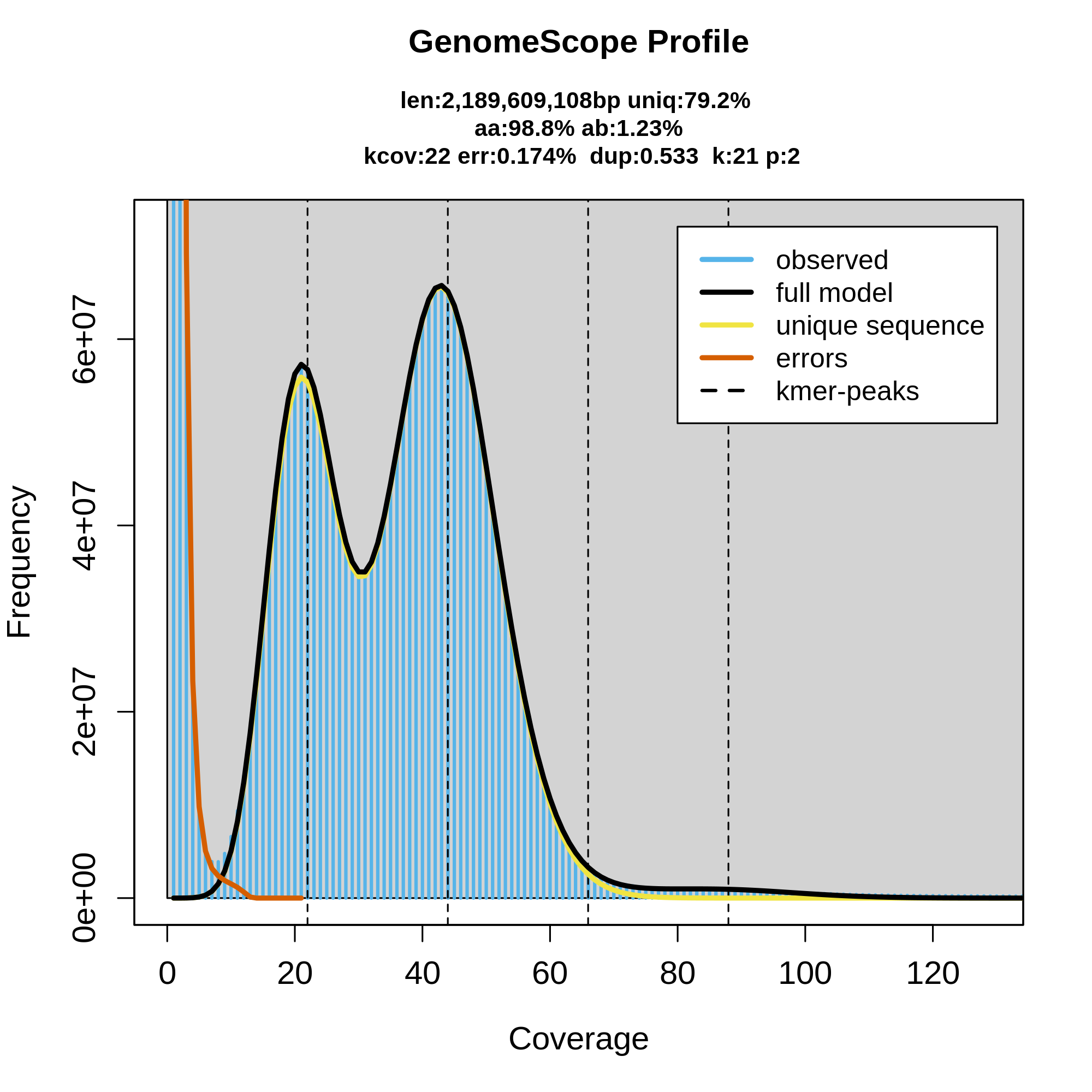
As you can see here, GenomeScope can be useful for getting an idea of what your raw dataset looks like, as well as feeling out the genome that should be represented by those sequencing reads. This can be useful as a QC step before even running the assembly, to make sure that your dataset is good enough to use. Here's an example of a good diploid dataset of HiFi reads:

How does the data look? What does the coverage look to be? How many peaks are there in the data and what do they represent? What are some characteristics of the genome as inferred by GenomeScope?

This data looks good, and you know that 1) because this tutorial text already called it good previously, and 2) there's a good amount of coverage, around 40X diploid coverage in fact. Additionally, the peaks are all very clear and distinct from each other and from the error k-mer slope on the left. Recall that the first peak represents haploid coverage (i.e., coverage of heterozygous loci) and the second peak is diploid coverage. GenomeScope is predicting the total size of the genome to be about 2.2 Gbp with 1.23% heterozygosity. This is data for Microtus pennsylvaticus, the eastern meadow vole.

Here's an example of another HiFi dataset:

Compare this to the previous examples. Does this look like a good dataset? Ignoring how GenomeScope itself is getting confused and can't get its model to fit properly to the k-mer spectra, let's look at the actual observed k-mer spectra. It does look like there's potentially two peaks whose distributions are overlapping, one peak around 10X and the other just under 20X. These are presumably our haploid and diploid peaks, but there's not enough coverage to resolve them properly here. This is an example of a GenomeScope QC that would tell me we don't have enough HiFi data to continue onto assembly, let's try to generate some more data.

Wow, more data! This result is from after adding one more (notably more successful) SMRT cell of HiFi data and re-running GenomeScope. We can see the resolution of the peaks much more cleanly, and the GenomeScope model fits the data much better now, so we can trust the genome characteristic estimates here more than before. If you noted the comparatively small genome size and wondered what this was, it's Anadara tuberculosa, the piangua.

Now you might be wondering: what happens if I try to assemble data without enough coverage? Answer: a headache. The assembly that results from the dataset that made the first GenomeScope plot resulted in two haplotypes of over 3,000 contigs each, which is very fragmented for a genome this small, recapitulated by their auN values being ~0.5 Mbp. In comparison, an assembly with the dataset pictured in the second GenomeScope plot resulted in two haplotypes of 500-800 contigs with auN values of 3.6-3.9 Mbp! The improvement in contiguity can also be visualized in the Bandage plots:

The above is the Hifiasm unitig graph for the assembly done without good HiFi coverage.

The above is the Hifiasm unitig graph for the assembly done with good (~56X) HiFi coverage.

Using Merqury in solo mode¶

Let's use Merqury on that database we just made to get the QV and some plots.

Use your text editor of choice to make a Slurm script (run_merqury.sl) to run the actual Merqury program with the following contents:

code

#!/bin/bash -e
#SBATCH --account       nesi02659
#SBATCH --job-name      merqury1
#SBATCH --cpus-per-task 8
#SBATCH --time          00:15:00
#SBATCH --mem           40G
#SBATCH --output        slurmlogs/%x.%j.log
#SBATCH --error         slurmlogs/%x.%j.err
#SBATCH --partition     milan

## load modules
module purge
module load Merqury
export MERQURY=/opt/nesi/CS400_centos7_bdw/Merqury/1.3-Miniconda3/merqury

## create solo merqury dir and use it
mkdir merqury_solo
cd merqury_solo

## run merqury
merqury.sh \
    ../read-db.meryl \
    ../assembly.fasta \
    output

cd -/lra

What's that export command doing there?

Merqury as a package ships with a lot of scripts, especially for plotting. The merqury.sh command that we're using is calling those scripts, but we need to tell it where we installed Merqury.

To find out the QV, we want the file named output.qv. Take a look at it and try to interpret the QV value you find (third column). If we recall the Phred scale system, this would mean that this QV value is great! Which is not surprising, considering we used HiFi data. It's worth noting, though, that we are using HiFi k-mers to evaluate sequences derived from those same HiFi reads. This does a good job of showing whether the assembly worked with that data well, but what if the HiFi data itself is missing parts of the genome, such as due to bias (e.g., GA dropout)? That's why it's important to use orthogonal datasets made using different sequencing technology, when possible. For instance, we can use an Illumina-based Meryl database to evaluate a HiFi assembly. For non-human vertebrates, this often results in the QV dropping from 50-60 to 35-45, depending on the genome in question.

Using Merqury in trio mode¶

So we just ran Merqury on our E. coli assembly, and evaluated it using the HiFi reads that we used for that assembly. Merqury can also utilize trio data (using those hapmer DBs we talked about before) to evaluate the phasing of an assembly, so let's try that with our HG002 trio data.

code

#!/bin/bash -e
#SBATCH --account       nesi02659
#SBATCH --job-name      merqury2
#SBATCH --cpus-per-task 8
#SBATCH --time          02:00:00
#SBATCH --mem           40G
#SBATCH --output        slurmlogs/%x.%j.log
#SBATCH --error         slurmlogs/%x.%j.err
#SBATCH --partition     milan

## load modules
module purge
module load Merqury
export MERQURY=/opt/nesi/CS400_centos7_bdw/Merqury/1.3-Miniconda3/merqury

## create trio merqury dir and use it
cd ~/lra/day3_assembly_qc
mkdir merqury_trio
cd merqury_trio
ln -s /nesi/nobackup/nesi02659/LRA/resources/assemblies/verkko/full/trio/assembly/assembly.*.fasta .
ln -s /nesi/nobackup/nesi02659/LRA/resources/maternal.k30.hapmer.meryl .
ln -s /nesi/nobackup/nesi02659/LRA/resources/paternal.k30.hapmer.meryl .

## let's run the program in a results directory to make things a little neater
mkdir results
cd results

## run merqury
merqury.sh \
    ../read-db.meryl \
    ../paternal.k30.hapmer.meryl \
    ../maternal.k30.hapmer.meryl \
    ../assembly.haplotype1.fasta \
    ../assembly.haplotype2.fasta \
    output

cd -/lra

You can also look in this folder for the merqury outputs if there isn't enough time to run the actual program: /nesi/nobackup/nesi02659/LRA/resources/merqury

There will be lots of outputs, but let's look at two now to get an idea for how the sequences have been partitioned between our assemblies, and whether that's consistent with information we know from trio sequencing. First let's look at the spectra-asm plot:

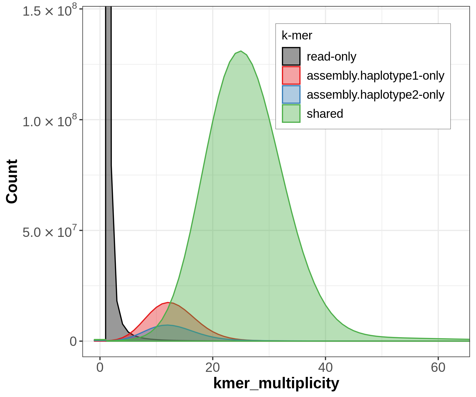
Merqury's spectra plots take the kmer spectrum (like you'd seen in GenomeScope) and color the kmers according to where the kmer is found: the reads only, one of the assemblies, or both of the assemblies.

A useful output from Merqury for evaluating phasing is the blob plot:

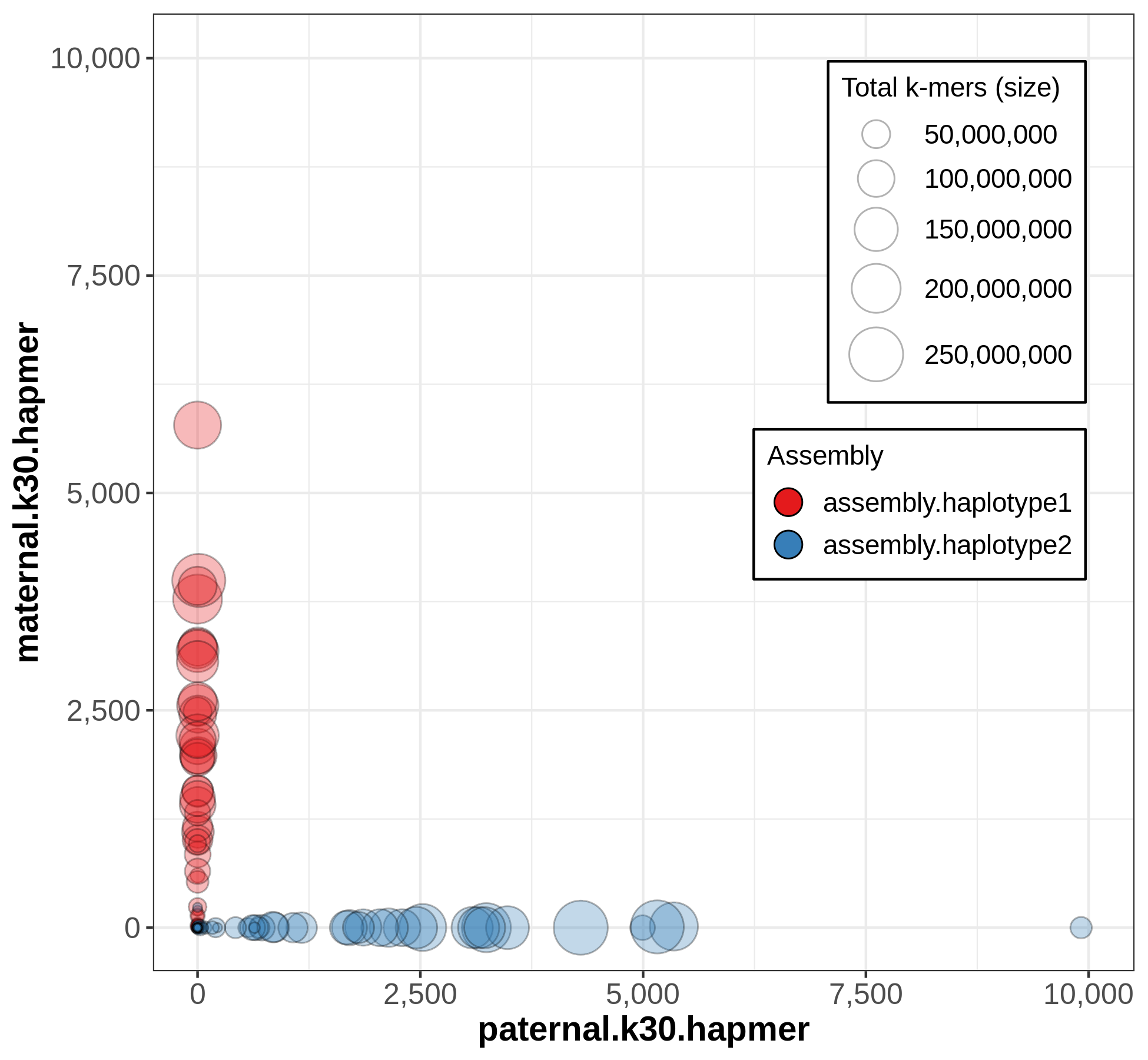
In this plot, each blob is a contig, and its x,y position represents parental hapmer content, while color represents assembly-of-origin.

What do different phasing approaches look like in Merqury?¶

Now we know what a nice trio-phased assembly looks like in Merqury, but what do the other options (Hi-C phasing or no phasing at all) look like? Let's look at an example from the zebra finch (Taeniopygia guttata), where the Vertebrate Genomes Project (VGP) has used hifiasm on the same HiFi dataset with different phasing approaches and evaluated the resulting assemblies with trio data in order to benchmark the different methods.

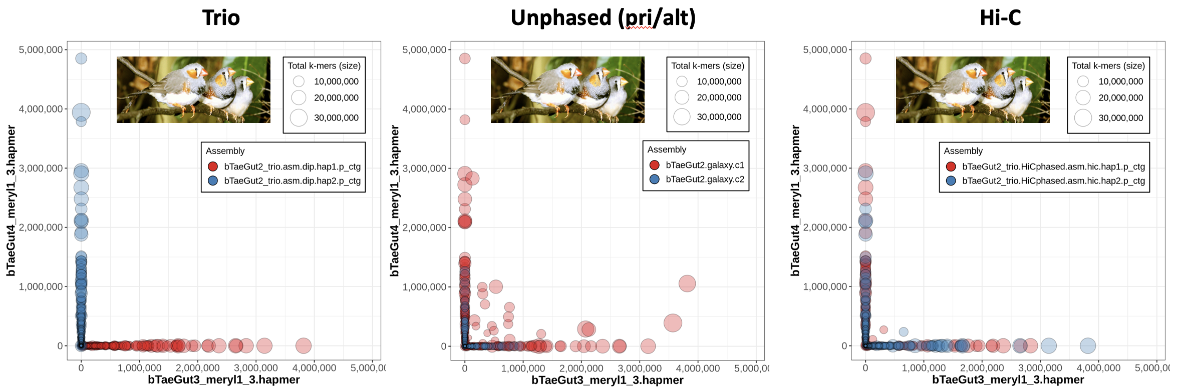
On the left, we have the blob plot for the trio assembly, which looks nicely phased as we expect -- all the contigs exhibit hapmers from only one parent (which you can tell because all blobs are along the x- or y- axis), and on top of that all the contigs from one assembly show only one parent's hapmers (i.e., hap1's red blobs all show only bTaeGut3 hapmers). In the middle, we have a blob plot for a primary/alternate set of assemblies generated without any phasing data. You'll notice that a lot of the primary assembly blobs are not on the axes, meaning they have hapmers from both parents.

Why are the alternate contigs all in phase?

It starts to make sense if you think about what the alternae assembly is meant to represent: the haplotigs. These are the alternate alleles for the heterozygous loci, so it would track that only one parent's hapmers are represented -- the alternate assembly is a collection of the "other side of the bubble"s when looking at the assembly graph.

The right plot is a blob plot from the Hi-C-phased assembly. Notably, most of the contigs are able to be properly phased, since they are almost all on the x- or -y axis.

Switch and Hamming errors using yak¶

Two more types of errors we use to assess assemblies are switch errors and Hamming errors. Hamming errors represent the percentage of SNPs wrongly phased (compared to ground truth), while switch errors represent the percentage of adjacent SNP pairs wrongly phased. See the following graphic:

As the image illustrates, switch errors occur when an assembly switches between haplotypes. These errors are more prevalent in pseudohaplotype (e.g., primary/alternate) assemblies that did not use any phasing data, as the assembler has no way of properly linking haplotype blocks, which can result in mixed hapmer content contigs that are a chimera of parental sequences.

code

#!/bin/bash -e
#SBATCH --account       nesi02659
#SBATCH --job-name      yaktrioeval
#SBATCH --cpus-per-task 32
#SBATCH --time          01:00:00
#SBATCH --mem           256G
#SBATCH --output        slurmlogs/%x.%j.log
#SBATCH --error         slurmlogs/%x.%j.err
#SBATCH --partition     milan

## change to qc dir, link things
cd ~/lra/day3_assembly_qc
ln -s /nesi/nobackup/nesi02659/LRA/resources/yak .
ln -s /nesi/nobackup/nesi02659/LRA/resources/assemblies/hifiasm/full/hic .
ln -s /nesi/nobackup/nesi02659/LRA/resources/assemblies/hifiasm/full/trio .
mkdir -p qc_yak
cd qc_yak

## load modules
module purge
module load yak

## run yak
yak trioeval -t 32 \
    ../yak/pat.HG003.yak ../yak/mat.HG004.yak \
    ../hic/HG002.hap1.fa.gz \
    > hifiasm.hic.hap1.trioeval

yak trioeval -t 32 \
    ../yak/pat.HG003.yak ../yak/mat.HG004.yak \
    ../trio/HG002.mat.fa.gz \
    > hifiasm.trio.mat.trioeval

Completeness (asmgene)¶

Another way to assess an assembly is via completeness, particularly with regard to expected gene content. If you have a reference genome that's been annotated with coding sequences, then you can use the tool asmgene to align multi-copy genes to your assembly and see if they remain multi-copy, or if the assembler has created a misassembly. asmgene works by aligning annotated transcripts to the reference genome, and record hits if the transcript is mapped at or over 99% identity over 99% or greater of the transcript length. If the transcript only has one hit, then it is single-copy (SC), otherwise it's multi-copy (MC). The same is then done for your assembly, and the fraction of missing multi-copy (%MMC) gene content is computed.

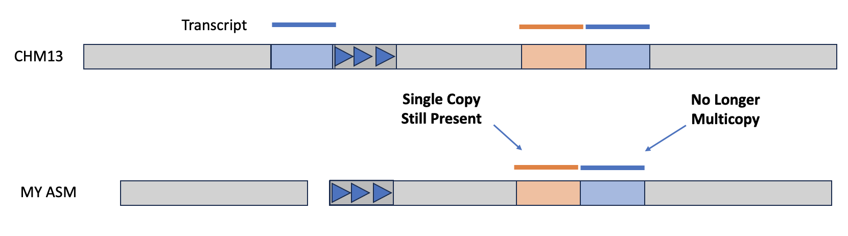
A perfect asesmbly would have %MMC be zero, while a higher fraction indicates the assembly has collapsed some of these multi-copy genes. Additionally, you can look at the presence (or absence!) of expected single-copy genes in order to check gene completeness of the assembly.

The output will be a tab-delimed list of metrics and the value of that metric for the reference and for your given assembly. The line full_sgl gives the number of single-copy genes present in the reference and your assembly—if these numbers are off-balanced, then you might have false duplications, which are also pointed out on the full_dup line. For the multi-copy genes, you can look at dup_cnt to see the number of multi-copy genes in the reference and see how many of those genes are still multi-copy in your assembly. You can then use these values to calculate %MMC via the formula 1 - (dup_cnt asm / dup_cnt ref).

Let's try running asmgene on haplotype1 and haplotype2 from the pre-baked Verkko trio assemblies.

code

## asmgene
cd ~/lra
mkdir -p day3_assembly_qc/asmgene
cd day3_assembly_qc/asmgene
# let's symlink some of the necessary files
ln -s /nesi/nobackup/nesi02659/LRA/resources/chm13/chm13v2.0.fa .
ln -s /nesi/nobackup/nesi02659/LRA/resources/chm13/CHM13-T2T.cds.fasta .
ln -s /nesi/nobackup/nesi02659/LRA/resources/assemblies/verkko/full/trio/assembly/assembly.haplotype1.fasta .
ln -s /nesi/nobackup/nesi02659/LRA/resources/assemblies/verkko/full/trio/assembly/assembly.haplotype2.fasta .

Now that we have our files, we're ready to go. Make a script with the following content and run it in the directory with the appropriate files:

code

#!/bin/bash -e
#SBATCH --account       nesi02659
#SBATCH --job-name      asmgene
#SBATCH --cpus-per-task 32
#SBATCH --time          05:00:00
#SBATCH --mem           256G
#SBATCH --output        slurmlogs/%x.%j.log
#SBATCH --error         slurmlogs/%x.%j.err
#SBATCH --partition     milan

## load modules
module purge
module load minimap2/2.24-GCC-11.3.0

## run minimap2 on ref, hap1, and hap2
minimap2 -cxsplice:hq -t32 \
    chm13v2.0.fa CHM13-T2T.cds.fasta \
    > ref.cdna.paf
minimap2 -cxsplice:hq -t32 \
    assembly.haplotype1.fasta CHM13-T2T.cds.fasta \
    > asm.hap1.cdna.paf
minimap2 -cxsplice:hq -t32 \
    assembly.haplotype2.fasta CHM13-T2T.cds.fasta \
    > asm.hap2.cdna.paf

## run asmgene

k8 /opt/nesi/CS400_centos7_bdw/minimap2/2.24-GCC-11.3.0/bin/paftools.js asmgene -a ref.cdna.paf asm.hap1.cdna.paf > verkko.haplotype1.asmgene.tsv
k8 /opt/nesi/CS400_centos7_bdw/minimap2/2.24-GCC-11.3.0/bin/paftools.js asmgene -a ref.cdna.paf asm.hap2.cdna.paf > verkko.haplotype2.asmgene.tsv

Tip

Another popular tool for checking genome completeness using gene content is the software Benchmarking Universal Single-Copy Orthologs (BUSCO). This approach uses a set of evolutionarily conserved genes that are expected to be present at single copy for a given taxa, so one could check their genome to see if, for instance, it has all the genes predicted to be necessary for Aves or Vertebrata. This approach is useful if your de novo genome assembly is for a species that does not have a reference genome yet. And it's even faster now with the recently developed tool minibusco!