Digging deeper 🪏

Key points 🔑

PCA is a way to visualise how similar or different samples are, taking into account all gene expression at once
In this dataset, PC1 (41% variance) separates treated vs untreated samples, while PC2 (26% variance) reflects cell-type differences
Raw counts need to be variance-stabilised with vst() before visualisation

Objectives 🎯

Explain what a PCA plot shows and how to interpret it in the context of RNA-seq
Create a DESeq2 object (dds) and apply variance stabilising transformation (vst())

We have 2 different conditions (treated with dexamethasone vs untreated control) and 4 different cell strains, and we want to explore how each of these could contribute to the overall gene expression profile of the sample.

Principal component analysis

A way to visualise sample-to-sample distances is a principal-components analysis (PCA). In this ordination method, the data points (i.e., here, the samples) are projected onto the 2D plane such that they spread out in the two directions which explain most of the differences in the data. The x-axis is the direction (or principal component) which separates the data points the most. The amount of the total variance which is contained in the direction is printed in the axis label.

In simple turns, we are making a plot that shows us how similar or different each sample, taking in to account all of the gene expression. A PCA plot can help us see the biggest sources of biological variation and help determine which has more of an affect on the gene expression – whether that be the treatment type, the cell type or something else.

install.packages("DESeq2")

library(DESeq2)
library(tidyverse)

We will use DEseq to to generate a special type of object in R, which will be called dds. This object can hold a lot of complex data types all in one. We will use it later for differential gene expression.

# first need to make gene ID a rowname rather than its own columns. 
countdata_fordds <- countdata_nozeros %>% 
  column_to_rownames("GeneID")

# now make the special deseq object, loading in counts and metadata and choosing the design
dds <- DESeqDataSetFromMatrix(countData = countdata_fordds, 
                              colData = coldata,
                              design = ~ cell + dex)

Warning in DESeqDataSet(se, design = design, ignoreRank): some variables in
design formula are characters, converting to factors

We can use the head() function to have a look at the counts in dds

head(counts(dds))

                S1-Un S2-Tr S3-Un S4-Tr S5-Un S6-Tr S7-Un S8-Tr
ENSG00000000003   679   448   873   408  1138  1047   770   572
ENSG00000000419   467   515   621   365   587   799   417   508
ENSG00000000457   260   211   263   164   245   331   233   229
ENSG00000000460    60    55    40    35    78    63    76    60
ENSG00000000938     0     0     2     0     1     0     0     0
ENSG00000000971  3251  3679  6177  4252  6721 11027  5176  7995

These are still the same as our original count data, we can check that by also running head on ‘countdata_fordds’ too.

head(countdata_fordds)

                S1-Un S2-Tr S3-Un S4-Tr S5-Un S6-Tr S7-Un S8-Tr
ENSG00000000003   679   448   873   408  1138  1047   770   572
ENSG00000000419   467   515   621   365   587   799   417   508
ENSG00000000457   260   211   263   164   245   331   233   229
ENSG00000000460    60    55    40    35    78    63    76    60
ENSG00000000938     0     0     2     0     1     0     0     0
ENSG00000000971  3251  3679  6177  4252  6721 11027  5176  7995

The creation of our dds “DESeqDataSeq” object earlier did not actually do anything yet to the data, it essentially loaded in and prepped it for further analysis.

As the counts in dds are raw counts, we need to first transform the counts for visualisation. We will use a function called vst() or variance stabilising transformation. This is a common type of transformation to use for visualising RNAseq data. We will make it in a new object called vsd, which will be a “DESeqTransform” object.

vsd <-  vst(dds)

Now we can make our PCA plot, using an all-in-one plotting function called plotPCA().

plotPCA(vsd, intgroup = c("dex", "cell"))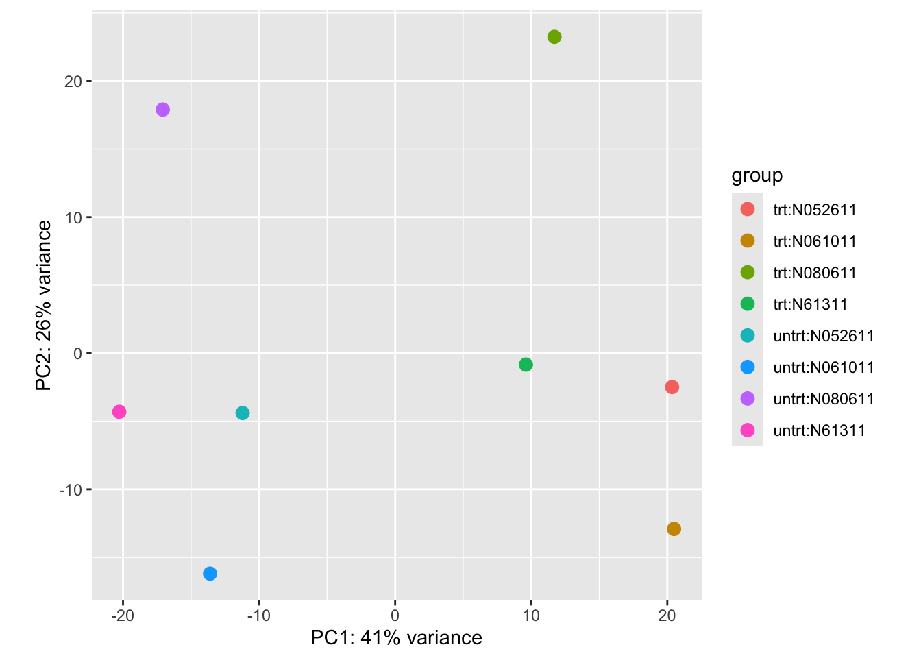

If the pca code above doesn’t work, try this:

pca_data <- plotPCA(vsd, intgroup = c("dex", "cell"), returnData = TRUE)

percentVar <- round(100 * attr(pca_data, "percentVar"))

ggplot(pca_data, aes(
  x = PC1,
  y = PC2,
  colour = dex,
  shape = cell
)) +
  geom_point(size = 3) +
  xlab(paste0("PC1: ", percentVar[1], "% variance")) +
  ylab(paste0("PC2: ", percentVar[2], "% variance")) +
  theme_classic()

This plot shows us that 41% of the variance is explained by principal component 1. We can see that this PC separates our two conditions, with all our treated samples on the right and our untreated samples on the left. We can also see that principal component 2 explains 26% of the variance, which explains a lot of the cell-specific genetic expression. The two samples from cell type ‘N080611’ appear to be the most different from the other cell types, sitting further away at the top of the plot. Together these two PCs explain 67% of the variance in gene expression - which is quite a lot! We can keep going further through the PCs – PC3, PC4, PC5 etc – and plot them too, but often the first PCs explain most of the variance.

Conclusion: treating with dexamethasone has a large effect on the gene expression, but the specific cell type also plays a role in the differences observed.