R Basics¶

Learning objectives

Key pointsObjectivesQuestions

Effectively using R is a journey of months or years. Still, you don't have to be an expert to use R, and you can start using and analyzing your data with about a day's worth of training.
It is important to understand how R organizes data in a given object type and how the mode of that type (e.g. numeric, character, logical, etc.) will determine how R will operate on that data.
Working with vectors effectively prepares you to understand how R organizes data.

Be able to create the most common R objects, such as vectors
Understand that vectors have modes, which correspond to the type of data they contain
Be able to use arithmetic operators on R objects
Be able to retrieve (subset), name, or replace values from a vector
Be able to use logical operators in a subsetting operation
Understand that lists can hold data of more than one mode and can be indexed

What will these lessons not cover?
What are the basic features of the R language?
What are the most common objects in R?

"The fantastic world of R awaits you" OR "Nobody wants to learn how to use R"¶

Before we begin this lesson, we want you to be clear on the goal of the workshop and these lessons. We believe that every learner can achieve competency with R. You have reached competency when you find that you are able to use R to handle common analysis challenges in a reasonable amount of time (which includes the time needed to look at learning materials, search for answers online, and ask colleagues for help). As you spend more time using R (there is no substitute for regular use and practice), you will gain competency and expertise. The more familiar you get, the more complex the analyses you will be able to carry out, with less frustration and in less time - the fantastic world of R awaits you!

What these lessons will not teach you¶

Nobody wants to learn how to use R. People want to learn how to use R to analyze their own research questions! Ok, maybe some folks learn R for R's sake, but these lessons assume that you want to start analyzing genomic data as soon as possible. Given this, there are many valuable pieces of information about R that we simply won't have time to cover. Hopefully, we will clear the hurdle of giving you just enough knowledge to be dangerous, which can be a high bar in R! We suggest you look into the additional learning materials in the tip box below.

Here are some R skills we will not cover in these lessons

How to create and work with R matrices
How to create and work with loops and conditional statements, and the "apply" family of functions (which are super useful, read more here)
How to do basic string manipulations (e.g. finding patterns in text using grep(), and replacing text using gsub())
How to plot using the default R graphic tools (we will cover plot creation, but will do so using the popular plotting package ggplot2)
How to use advanced R statistical functions

Where to learn more

The following are good resources for learning more about R. Some of them can be quite technical, but if you are a regular R user you may ultimately need this technical knowledge.

R for Beginners: By Emmanuel Paradis and a great starting point
The R Manuals: Maintained by the R project
R contributed documentation: Also linked to the R project; importantly there are materials available in several languages
R for Data Science: A wonderful collection by noted R educators and developers Garrett Grolemund and Hadley Wickham
Practical Data Science for Stats: Not exclusively about R usage, but a nice collection of pre-prints on data science and applications for R
Programming in R Software Carpentry lesson: There are several Software Carpentry lessons in R to choose from

Objects¶

Creating objects in R¶

Reminder

At this point you should be coding along in the genomics_r_basics.R script we created in the last episode. Writing your commands in the script (and commenting it) will make it easier to record what you did and why.

What might be called a variable in many languages is called an object in R.

To create an object, you need:

A name (e.g. a)
A value (e.g. 1)
The assignment operator (<-)

In your script, genomics_r_basics.R, use the R assignment operator <- to assign 1 to the object a as shown. Remember to leave a comment in the line above (using the #) to explain what you are doing:

r

# This line creates the object 'a' and assigns it the value '1'

a <- 1

Next, run this line of code in your script. You can run a line of code by hitting the Run button that is above the first line of your script in the header of the 'Source' pane or you can use the appropriate shortcut:

Windows execution shortcut: Ctrl + Enter
Mac execution shortcut: Cmd(⌘) + Enter

To run multiple lines of code, highlight all the line you wish to run and then hit Run or use the shortcut key combo listed above. In the RStudio 'Console', you should see:

a <- 1
>

The 'Console' will display lines of code run from a script and any outputs or status/warning/error messages (usually in red). In the 'Environment' window you will also get a table:

Values
a	1

The 'Environment' window allows you to keep track of the objects you have created in R.

Exercise: Create some objects in R

Create the following objects and give each object an appropriate name (your best guess at what name to use is fine):

Create an object that has the value of number of pairs of human chromosomes
Create an object that has a value of your favorite gene name
Create an object that has this URL as its value: "ftp://ftp.ensemblgenomes.org/pub/bacteria/release-39/fasta/bacteria_5_collection/escherichia_coli_b_str_rel606/"
Create an object that has the value of the number of chromosomes in a diploid human cell

Solution

Here as some possible answers to the challenge:

human_chr_number <- 23
gene_name <- 'pten'
ensemble_url <- "ftp://ftp.ensemblgenomes.org/pub/bacteria/release-39/fasta/bacteria_5_collection/escherichia_coli_b_str_rel606/"
human_diploid_chr_num <-  2 * human_chr_number

Naming objects in R¶

Here are some important details about naming objects in R

Avoid spaces and special characters
Object names cannot contain spaces or the minus sign (-). You can use _ to make names more readable. You should avoid using special characters in your object name (e.g. ! @ # . , etc.). Also, object names cannot begin with a number.
Use short, easy-to-understand names
Avoid naming your objects using single letters (e.g. n, p, etc.). This is mostly to encourage you to use names that would make sense to anyone reading your code (a colleague, or even yourself a year from now). Also, avoiding excessively long names will make your code more readable.
Avoid commonly used names
Several names may already have a definition in the R language (e.g. mean, min, max). One clue that a name already has meaning is that if you start typing a name in RStudio and it gets a colored highlight or RStudio gives you a suggested autocompletion, you have chosen a name that has a reserved meaning.
Use the recommended assignment operator
In R, we use <- as the preferred assignment operator. = works too, but is most commonly used in passing arguments to functions (more on functions later). Shortcuts for the R assignment operator are:
- Windows execution shortcut: Alt + -
- Mac execution shortcut: Option + -

There are a few more suggestions about naming and style you can learn more about as you write more R code. Several "style guides" have advice, and one to start with is the tidyverse R style guide.

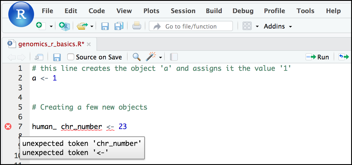
Pay attention to warnings in the 'Source' panel

If you enter a line of code in your script that contains an error, RStudio may give you an error message and underline this mistake. Sometimes, these messages are easy to understand, but often, the messages may need some figuring out. Paying attention to these warnings will help you avoid mistakes. In the example below, our object name has a space, which is not allowed in R. The error message does not say this directly, but R is "not sure" about how to assign the number to human_ chr_number when the object name we want is human_chr_number

Reassigning object names or deleting objects¶

Once an object has a value, you can change that value by overwriting it. R will not give you a warning or error if you overwrite an object, which may or may not be a good thing depending on how you look at it.

r

# gene_name has the value 'pten' or whatever value you used in the challenge
# We will now assign the new value 'tp53'

gene_name <- 'tp53'

You can also remove an object from R's memory entirely. The rm() function will delete the object.

r

# Delete the object 'gene_name'
rm(gene_name)

If you run a line of code that has only an object name, R will normally display the contents of that object. In this case, we are told the object no longer exists.

r

gene_name

Error

Error: object 'gene_name' not found

Understanding object data types (modes)¶

In R, every object has two properties:

Length: The number of distinct values are held in that object
Mode: The classification (type) of that object

We will get to the "length" property later in the lesson. The "mode" property corresponds to the type of data an object represents. The most common modes you will encounter in R are:

Mode (abbreviation)	Type of data
Numeric (`num`)	Numbers such as floating point (i.e. decimals, e.g. 1.0, 0.5, 3.14). There are also more specific numeric types (`dbl` - Double, `int` - Integer). These differences are not relevant for most beginners and pertain to how these value are stored in memory
Character (`chr`)	A sequence of letters/numbers in single `''` or double `""` quotes
Logical (`logi`)	Boolean values `TRUE` or `FALSE`

There are a few other modes (i.e. "complex", "raw" etc.) but these are the three we will work with in this lesson.

Data types are common across many programming languages, but also in natural language, where we refer to them as the parts of speech, e.g. nouns, verbs, adverbs, etc. Once you know if a word - perhaps an unfamiliar one - is a noun, you can probably guess you can count it and make it plural if there is more than one (e.g. 1 Tuatara, or 2 Tuataras). If something is an adjective, you can usually change it into an adverb by adding "-ly" (e.g., jejune vs. jejunely). Depending on the context, you may need to decide if a word is in one category or another (e.g "cut" may be (1) a noun when it's on your finger or (2) a verb when you are preparing vegetables). These concepts have important analogies when working with R objects.

Exercise: Create objects and check their modes

Create the following objects in R, then verify their modes using the mode() function. Try to guess what the mode will be before you look at the solution.

chromosome_name <- 'chr02'
od_600_value <- 0.47
chr_position <- '1001701'
spock <- TRUE
pilot <- Earhart

Solution

mode(chromosome_name) 
mode(od_600_value) 
mode(chr_position) 
mode(spock) 
mode(pilot)

[1] "character"
[1] "numeric"
[1] "character"
[1] "logical"
Error: object 'pilot' not found

Notice from the solution that even if a series of numbers is given as a value R will consider them to be in the "character" mode if they are enclosed with single or double quotes. Also, notice that you cannot take a string of alphanumeric characters (i.e., Earhart) and assign it as a value for an object. In this case, R looks for an object named Earhart, but since there is no object, no assignment can be made. If Earhart did exist, then the mode of pilot would be whatever the mode of Earhart was originally. If we want to create an object called pilot that was the name "Earhart", we need to enclose Earhart in quotation marks.

r

pilot <- "Earhart"
mode(pilot)

Mathematical and functional operations on objects¶

Once an object exists (which, by definition, also means it has a mode), R can manipulate that object using appropriate methods. For example, objects of the numeric modes can be added, multiplied, divided, etc. R provides several mathematical (arithmetic) operators including:

Operator	Description
`+`	Addition
`-`	Subtraction
`*`	Multiplication
`/`	Division
`^` or `**`	Exponentiation
`%/%`	Integer division (division where the remainder is discarded)
`%%`	Modulus (returns the remainder after division)

These can be used with literal numbers:

r

(1 + (5 ** 0.5))/2

and importantly, can be used on any object that evaluates to (i.e. interpreted by R) a numeric object:

r

human_chr_number <- 23

# Multiply the object 'human_chr_number' by 2
human_chr_number * 2

Exercise: Compute the golden ratio

One approximation of the golden ratio ($\phi$) can be found by taking the sum of 1 and the square root of 5, and dividing by 2 as in the example above.

\[ \phi = \frac{1 + \sqrt{5}}{2} \]

Compute the golden ratio to 3 digits of precision using the sqrt() and round() functions.

Hint: Remember the round() function can take two arguments.

Solution

round((1 + sqrt(5))/2, digits = 3)

# Notice that you can place one function inside of another.

Vectors¶

Vectors are probably the most commonly used object type in R. A vector is a collection of values that are all of the same type (numbers, characters, etc.). One of the most common ways to create a vector is to use the c() function — the "concatenate" or "combine" function. Inside the function you may enter one or more values; for multiple values, separate each value with a comma:

r

# Create the SNP gene name vector
snp_genes <- c("OXTR", "ACTN3", "AR", "OPRM1")

Vectors always have a mode and a length. You can check these with the mode() and length() functions respectively. Another useful function that gives both of these pieces of information is the str() (structure) function.

r

# Check the mode, length, and structure of 'snp_genes' 
mode(snp_genes) 
length(snp_genes) 
str(snp_genes)

Vectors are very important in R. Another data type that we will work with later in this lesson, data frames, are collections of vectors. What we learn here about vectors will pay off even more when we start working with data frames.

Creating and subsetting vectors¶

Let's create a few more vectors to play around with:

r

# Some interesting human SNPs
# While accuracy is important, typos in the data won't hurt you here

snps <- c("rs53576", "rs1815739", "rs6152", "rs1799971")
snp_chromosomes <- c("3", "11", "X", "6") 
snp_positions <- c(8762685, 66560624, 67545785, 154039662)

Once we have vectors, one thing we may want to do is retrieve one or more values from our vector. To do so, we use bracket notation. We type the name of the vector followed by square brackets. In those square brackets we place the index (i.e., a number that corresponds to the position of the value in the vector) in that bracket as follows:

r

# Get the 3rd value in the 'snps' vector
snps[3]

In R, every item in your vector is indexed, starting from the first item (1) through to the final number of items in your vector. You can also retrieve a range of numbers:

r

# Get the 1st to 3rd value in the 'snps' vector

snps[1:3]

If you want to retrieve several (but not necessarily sequential) items from a vector, you pass a vector of indices (i.e., a vector that has the numbered positions of the elements you wish to retrieve).

r

# Get the 1st, 3rd, and 4th value in the 'snps' vector

snps[c(1, 3, 4)]

There are additional (and perhaps less commonly used) ways of subsetting a vector (see these examples). Several of these subsetting expressions can be combined:

r

# Get the 1st through the 3rd value, and 4th value in the 'snps' vector
# Yes, this is a little silly in a vector of only 4 values.

snps[c(1:3, 4)]

Adding to, removing, or replacing values in existing vectors¶

Once you have an existing vector, you may want to add a new item to it. To do so, you can use the c() function again to add your new value:

r

# Add the gene "CYP1A1" and "APOA5" to our 'snp_genes' vector
# Note: This overwrites our existing vector.

snp_genes <- c(snp_genes, "CYP1A1", "APOA5")

We can verify that "snp_genes" contains the new gene entry

r

snp_genes

Output

[1] "OXTR"   "ACTN3"  "AR"     "OPRM1"  "CYP1A1" "APOA5"

Using a negative index will return a version of a vector with that index's value removed:

r

snp_genes[-6]

Output

[1] "OXTR"   "ACTN3"  "AR"     "OPRM1"  "CYP1A1"

We can remove that value from our vector by overwriting it with this expression:

r

snp_genes <- snp_genes[-6]

snp_genes

Output

[1] "OXTR"   "ACTN3"  "AR"     "OPRM1"  "CYP1A1"

We can also explicitly rename or add a value to our index using bracket notation:

r

snp_genes[7] <- "APOA5"

snp_genes

Output

[1] "OXTR"   "ACTN3"  "AR"     "OPRM1"  "CYP1A1" NA       "APOA5"

Filling in the blanks

Notice in the example above that there is an NA in the 6^th position of the vector? Recall that R keeps track of every element in vectors by numeric indexing. This means that when we added a 7^th element where there is no 6^th element, R fills it with NA which functionally means "missing value" or "Not Available".

Exercise: Examining and subsetting vectors

Answer the following question to test your knowledge of vectors

Which of the following are true of vectors in R?

A) All vectors have a mode or a length
B) All vectors have a mode and a length
C) Vectors may have different lengths
D) Items within a vector may be of different modes
E) You can use the c() to add one or more items to an existing vector
F) You can use the c() to add a vector to an exiting vector

Solution

A) False - Vectors have both of these properties
B) True
C) True
D) False - Vectors have only one mode (e.g. numeric, character); all items in a vector must be of this mode.
E) True
F) True

Logical subsetting¶

There is one last set of cool subsetting capabilities we want to introduce. It is possible within R to retrieve items in a vector based on a logical evaluation or numerical comparison. For example, let's say we wanted get all of the SNPs in our vector of SNP positions that were greater than 100,000,000. We could index using the > (greater than) logical operator:

r

snp_positions[snp_positions > 100000000]

Output

[1] 154039662

In the square brackets you place the name of the vector followed by the comparison operator and (in this case) a numeric value. Some common logical operators in R are:

Operator	Description
`<`	Less than
`<=`	Less than or equal to
`>`	Greater than
`>=`	Greater than or equal to
`==`	Exactly equal to
`!=`	Not equal to
`!x`	Not x
`a \| b`	a or b
`a & b`	a and b

The magic of programming

The reason why the expression snp_positions[snp_positions > 100000000] works can be better understood if you examine what the expression snp_positions > 100000000 evaluates to:

r

snp_positions > 100000000

Output

[1] FALSE FALSE FALSE  TRUE

The output above is a logical vector where the 4^th element is TRUE. When you pass a logical vector as an index, R will return values that are or evaluate to TRUE:

r

snp_positions[c(FALSE, FALSE, FALSE, TRUE)]

Output

[1] 154039662

If you have never coded before, this type of situation starts to expose the “magic” of programming. We mentioned before that in the bracket notation you take your named vector followed by brackets which contain an index: named_vector[index]. The “magic” is that the index needs to evaluate to a number. So, even if it does not appear to be an integer (e.g. 1, 2, 3), as long as R can evaluate it, we will get a result. That our expression snp_positions[snp_positions > 100000000] evaluates to a number can be seen in the following situation. If you wanted to know which index (1, 2, 3, or 4) in our vector of SNP positions was the one that was greater than 100,000,000? We can use the which() function to return the indices of any item that evaluates as TRUE in our comparison:

r

which(snp_positions > 100000000)

Output

[1] 4

Why this is important

Often in programming we will not know what inputs and values will be used when our code is executed. Rather than put in a pre-determined value (e.g 100000000) we can use an object that can take on whatever value we need. So for example:

r

snp_marker_cutoff <- 100000000
snp_positions[snp_positions > snp_marker_cutoff]

Output

[1] 154039662

Ultimately, it’s putting together flexible, reusable code like this that gets at the “magic” of programming!

A few final vector tricks¶

Finally, there are a few other common retrieve or replace operations you may want to know about. First, you can check to see if any of the values of your vector are missing (i.e. are NA, that stands for "Not Available"). Missing data will get a more detailed treatment later, but the is.na() function will return a logical vector, with TRUE for any NA value:

r

# Current value of 'snp_genes' inspected using 'str()':
# chr [1:7] "OXTR" "ACTN3" "AR" "OPRM1" "CYP1A1" NA "APOA5"

is.na(snp_genes)

Output

[1] FALSE FALSE FALSE FALSE FALSE  TRUE FALSE

Sometimes, you may wish to find out if a specific value (or several values) is present in a vector. You can do this using the comparison operator %in%
which will return TRUE for any value in the vector you are searching:

r

# Current value of 'snp_genes' inspected using 'str()':
# chr [1:7] "OXTR" "ACTN3" "AR" "OPRM1" "CYP1A1" NA "APOA5"

# Test to see if "ACTN3" or "APO5A" is in the snp_genes vector
# If you are looking for more than one value, you must pass this as a vector

c("ACTN3","APOA5") %in% snp_genes

Output

[1] TRUE TRUE

Lists¶

Lists are another form of data structure in R. Although it resembles vectors, two key properties differentiates them and make lists extremely useful for more complex data storage:

Lists can contain data of multiple modes
Remember that vectors can only contain data of one mode.
Lists can be nested
This means that a list can contain other lists. Vectors, on the other hand, are flat (i.e., all values of a vector is laid out on a single level)

Due to their flexibility, many complex analyses store data/return results using lists.

Attribution

Some of the content here was adapted from an excellent tutorial which we highly recommend you read.

Creating lists¶

Let's begin by creating a list using existing vectors created prior.

r

# We will replace the vector 'snp_genes' to its original values
snp_genes <- c("OXTR", "ACTN3", "AR", "OPRM1")

# Create a list
snps_list <- list(
  genes = snp_genes,
  reference_snps = snps,
  chromosomes = snp_chromosomes,
  positions = snp_positions
)

Copy-pasting code

Make sure to highlight, copy, paste, then run all lines of the "Create a list" code block.

We can see how R prints a list by calling it.

r

snps_list

Output

$genes
[1] "OXTR"  "ACTN3" "AR"    "OPRM1"

$reference_snps
[1] "rs53576"   "rs1815739" "rs6152"    "rs1799971"

$chromosomes
[1] "3"  "11" "X"  "6" 

$positions
[1]   8762685  66560624  67545785 154039662

Here, we have a named list that contains the vectors genes, reference_snps, chromosomes, and positions. We can also inspect the modes of data stored in the list using str().

r

str(snps_list)

Output

List of 4
 $ genes         : chr [1:4] "OXTR" "ACTN3" "AR" "OPRM1"
 $ reference_snps: chr [1:4] "rs53576" "rs1815739" "rs6152" "rs1799971"
 $ chromosomes   : chr [1:4] "3" "11" "X" "6"
 $ positions     : num [1:4] 8.76e+06 6.66e+07 6.75e+07 1.54e+08

Unnamed items in a list

When we created our list, we assigned a name to each item within the list. However, this is not strictly necessary. Let's try it out and see what happens:

r

# Create the list
unnamed_snps_list <- list(
  snp_genes,
  snps,
  snp_chromosomes,
  snp_positions
)

# Call the list
unnamed_snps_list

Output

[[1]]
[1] "OXTR"  "ACTN3" "AR"    "OPRM1"

[[2]]
[1] "rs53576"   "rs1815739" "rs6152"    "rs1799971"

[[3]]
[1] "3"  "11" "X"  "6" 

[[4]]
[1]   8762685  66560624  67545785 154039662

Notice that the items are not named and are simply given a numeric index within double square brackets [[1]]. In fact, you can create a list with a mixture of named and unnamed items. While this is still a valid way to create lists, it is not very user-friendly as we have no way of telling what information is stored in each of the items. Ideally, you should assign names to each item in the list when creating it to easily identify the kinds of information stored within it.

Importance of correct symbols for adding items to lists

Notice that we have used the assignment operator <- to create snps_list and the equal symbol = to add vectors to each item in the list. When creating a vector, you can use either symbol to achieve the same goal. However, when creating lists, the distinction between symbols is NOT a stylistic choice and will affect the output. We can see what happens if we were to change the = operator to <- within the brackets.

r

wrong_operator <- list(
  genes <- snp_genes,
  reference_snps = snps,
  chromosomes = snp_chromosomes,
  positions = snp_positions
)

# Call the list
wrong_operator

Output

[[1]]
[1] "OXTR"  "ACTN3" "AR"    "OPRM1"

$reference_snps
[1] "rs53576"   "rs1815739" "rs6152"    "rs1799971"

$chromosomes
[1] "3"  "11" "X"  "6" 

$positions
[1]   8762685  66560624  67545785 154039662

We can observe two things:

The name for the first list item genes is now simply a numeric index [[1]]
There is an additional object in the global environment called genes

Switching the assignment operator adds an unnamed item in the list, and creates a vector object called genes in the global environment. Make certain to use the correct operator when creating lists to avoid unintentionally populating your working environment.

Refer to items in a list¶

In the examples above, we refer to values in a vector using their indices (e.g. vector[c(2, 3)]). For the named list we created, we can refer to the name of the items themselves. Commonly, this is done using the $ like so: list_name$object_name. For example, we can retrieve gene positions from snps_list:

r

snps_list$positions

Output

[1]   8762685  66560624  67545785 154039662

There are also ways to refer to objects in a list using square brackets [] (like for vectors). However, this method is more complex. This section of the linked tutorial provides a good analogy on how the brackets are interpreted in R in the context of lists.

Add or replace items in a list¶

We can also add items to lists. Let's add a logical vector to the list.

r

# Create logical vector
snps_DE <- c(TRUE, FALSE, FALSE, TRUE)

# Add to list
snps_list$DE_genes <- snps_DE

# Inspect list
str(snps_list)

Output

List of 5
 $ genes         : chr [1:4] "OXTR" "ACTN3" "AR" "OPRM1"
 $ reference_snps: chr [1:4] "rs53576" "rs1815739" "rs6152" "rs1799971"
 $ chromosomes   : chr [1:4] "3" "11" "X" "6"
 $ positions     : num [1:4] 8.76e+06 6.66e+07 6.75e+07 1.54e+08
 $ DE_genes      : logi [1:4] TRUE FALSE FALSE TRUE

Now, snps_list has 5 items, the last of which is a logical vector that we just added.

To replace items in a list, we refer to the item, then assign it something else. Let's say we want the DE_genes to be in numeric, instead of logical mode.

r

# Replace DE_genes with a character vector
snps_list$DE_genes <- as.numeric(snps_DE)

# Inspect list
str(snps_list)

Output

List of 5
 $ genes         : chr [1:4] "OXTR" "ACTN3" "AR" "OPRM1"
 $ reference_snps: chr [1:4] "rs53576" "rs1815739" "rs6152" "rs1799971"
 $ chromosomes   : chr [1:4] "3" "11" "X" "6"
 $ positions     : num [1:4] 8.76e+06 6.66e+07 6.75e+07 1.54e+08
 $ DE_genes      : num [1:4] 1 0 0 1

Notice that DE_genes has turned into numeric mode from its original logical mode, where TRUE is 1 and FALSE is 0.

Up till now, we have made a list that contain items with a vector length of 4. There is no requirement that all items in lists to must have the same length. Lists can have any number of items of different lengths. For example, let's add a single number into the list:

r

# Add a number to the list
snps_list$sig_threshold <- 0.05

# Inspect list
str(snps_list)

Output

List of 6
 $ genes         : chr [1:4] "OXTR" "ACTN3" "AR" "OPRM1"
 $ reference_snps: chr [1:4] "rs53576" "rs1815739" "rs6152" "rs1799971"
 $ chromosomes   : chr [1:4] "3" "11" "X" "6"
 $ positions     : num [1:4] 8.76e+06 6.66e+07 6.75e+07 1.54e+08
 $ DE_genes      : num [1:4] 1 0 0 1
 $ sig_threshold : num 0.05

Subset or remove objects from a list¶

Single square brackets [] can be used to subset a list based on the item's index or name. The following code will subset the items genes, reference_snps, and sig_threshold from snps_list.

r

# Method 1: Use index
# We know the index of genes (1), reference_snps (2) and sig_threshold (6). 
sub_snps_list <- snps_list[c(1:2, 6)]

# Inspect list
str(sub_snps_list)

Output

List of 3
 $ genes         : chr [1:4] "OXTR" "ACTN3" "AR" "OPRM1"
 $ reference_snps: chr [1:4] "rs53576" "rs1815739" "rs6152" "rs1799971"
 $ sig_threshold : num 0.05

r

# Method 2: Use names
sub_snps_list <- snps_list[c("genes", "reference_snps", "sig_threshold")]

# Inspect list
str(sub_snps_list)

Output

List of 3
 $ genes         : chr [1:4] "OXTR" "ACTN3" "AR" "OPRM1"
 $ reference_snps: chr [1:4] "rs53576" "rs1815739" "rs6152" "rs1799971"
 $ sig_threshold : num 0.05

List bracket notation

When subsetting a list using single square brackets [], the result is always a list. To access the vector directly, we need to use double square brackets [[]]. For example:

r

# Return the vector in a list
snps_list["chromosomes"]

# Return the vector directly
snps_list[["chromosomes"]]

Output

$chromosomes
[1] "3"  "11" "X"  "6"

[1] "3"  "11" "X"  "6"

To remove objects in a list, we first refer to it, then assign it as NULL.

r

# Remove sig_threshold
sub_snps_list$sig_threshold <- NULL

# Inspect list
str(sub_snps_list)

Output

List of 2
 $ genes         : chr [1:4] "OXTR" "ACTN3" "AR" "OPRM1"
 $ reference_snps: chr [1:4] "rs53576" "rs1815739" "rs6152" "rs1799971"

Et voilà! The numeric vector sig_threshold is no longer a part of sub_snps_list.

Nested list¶

A defining feature of lists is that it can be nested (i.e., lists can be stored inside of a list). This property allows the storage of data that are structured hierarchically or in a tree-like fashion (i.e., dendrograms). It is also useful for storing different types of data in an organised manner (e.g., a list of model values with a nested list that contains sample information or metadata). You will undoubtedly encounter complex nested list structures in your R journey. The majority of the time, we are only concerned with referring to or subsetting nested lists. With that in mind, let's start with creating a nested list followed by an example on subsetting.

r

# Create nested list
nested_snps_list <- list(
  gene = snp_genes,
  snp_info = list(
    reference = snps,
    chromosome = snp_chromosomes,
    position = snp_positions
  ),
  result = list(
    DE = snps_DE,
    threshold = 0.05
  ),
  metadata = list(
    sample_group = list(
      A = c("S1", "S2"),
      B = "S3",
      C = "S4"
    )
  )
)

Reminder

Again, make sure to highlight, copy, paste, and run the entire code block!

Inspect the list structure:

r

str(nested_snps_list)

Output

List of 4
 $ gene    : chr [1:4] "OXTR" "ACTN3" "AR" "OPRM1"
 $ snp_info:List of 3
  ..$ reference : chr [1:4] "rs53576" "rs1815739" "rs6152" "rs1799971"
  ..$ chromosome: chr [1:4] "3" "11" "X" "6"
  ..$ position  : num [1:4] 8.76e+06 6.66e+07 6.75e+07 1.54e+08
 $ result  :List of 2
  ..$ DE       : logi [1:4] TRUE FALSE FALSE TRUE
  ..$ threshold: num 0.05
 $ metadata:List of 1
  ..$ sample_group:List of 3
  .. ..$ A: chr [1:2] "S1" "S2"
  .. ..$ B: chr "S3"
  .. ..$ C: chr "S4"

Phew! There's quite a bit of information here! Let's break it down.

We have created a list with 4 objects, each of which contain different objects and modes: list, character, numeric, and logical.
snp_info and result are nested lists with structures we have encountered before.
- They each have vectors of varying modes.
- result has vectors of varying lengths.
The nested list metadata is the parent of sample_group.
- sample_group has children A, B, and C, all of which are character vectors.

Now we can subset/retrieve some of the information in the nested list. As we are working with named lists (and sub-lists), it is easier to use the $ method. Let's subset the chromosome vector

r

nested_snps_list$snp_info$chromosome

Output

[1] "3"  "11" "X"  "6"

If you want to use the index and square brackets method:

r

nested_snps_list[[2]][[2]]

Output

[1] "3"  "11" "X"  "6"

You can read the above code as "the second item (here, a character vector) of the second item (a list)"

You can retrieve objects from deeply nested lists as long as you know the object's name or index, and how it is structured (parent-child hierarchy).

Review exercises¶

Exercise 1

What data modes are the following vectors?

a. snps
b. snp_chromosomes
c. snp_positions

Solution

Use mode() to find out.

a. Character
b. Character
c. Numeric

Exercise 2

Add the following values to the specified vectors:

a. To the snps vector add: “rs662799”
b. To the snp_chromosomes vector add: 11
c. To the snp_positions vector add: 116792991

Solution

# Answer (a)
snps <- c(snps, "rs662799")

# Answer (b)
snp_chromosomes <- c(snp_chromosomes, "11") # Did you use quotes?

# Answer (c)
snp_positions <- c(snp_positions, 116792991)

Exercise 3

Make the following change to the snp_genes vector:

Hint: Your vector should look like this in ‘Environment’:
chr [1:7] "OXTR" "ACTN3" "AR" "OPRM1" "CYP1A1" NA "APOA5".
If not recreate the vector by running this:

r

snp_genes <- c("OXTR", "ACTN3", "AR", "OPRM1", "CYP1A1", NA, "APOA5")

a. Create a new version of snp_genes that does not contain "CYP1A1" and then
b. Add 2 NA values to the end of snp_genes

Solution

# Answer (a)
snp_genes <- snp_genes[-5]
# or use logical subsetting
snp_genes <- snp_genes[snp_genes != "CYP1A1"]

# Answer (c)
snp_genes <- c(snp_genes, NA, NA)

Exercise 4

Using indexing, create a new vector named combined that contains:

The the 1^st value in snp_genes
The 1^st value in snps
The 1^st value in snp_chromosomes
The 1^st value in snp_positions

Solution

combined <- c(
  snp_genes[1], 
  snps[1], 
  snp_chromosomes[1], 
  snp_positions[1]
)

Exercise 5

What type of data is combined?

Solution

It is a character vector. Use typeof() to find out.