Relational data

Lesson objectives

• Understand the concepts in relational data
• Use left_join() to join two tables based on shared keys
• Understand the different join functions

A brief introduction to relational data

Data analysis rarely involves only one data source. In many cases, insightful conclusions (and hypotheses) can only be gleaned and built by combining data from multiple sources. Collectively, this type of data is termed relational data, where the relationships between data points are of primary importance. Relational data is widespread in biology and you have probably encountered and generated it during your research. The table below outlines some cases where relational data can arise from:

Case	Example scenario
Subjecting the same data to different types of analyses	Based on an amino acid sequence, predict signal peptide sequences, active site motifs, and secondary structures using different software.
Collecting and analysing different data from the same sample.	Correlate chemical measurements of different metabolites with sequence variants within a population.
Comparing your data with data available in the literature or public databases.	Identify homology between your set of sequences and those in NCBI’s RefSeq and then query the sequence’s role in metabolism via gene ontology.

Almost all modern databases rely on concepts derived from relational data. For example, searching for something in NCBI will return matches across various databases (e.g., Gene, Protein, Nucleotide, etc.). When you access one of the records you will see links to other NCBI databases for that record (e.g., Taxonomy, Conserved Domains, BioProjects, etc.). Moreover, the use of controlled vocabulary across biological databases (e.g., KEGG orthology (KO), enzyme commission (EC) numbers, transporter classification (TC) numbers, GO IDs, etc.) has made it easier to cross-reference information stored in other databases.

The key(s) to relational data

An essential characteristic of relational data is that data across multiple tables are connected via keys. You can think of keys as IDs. When analysing tabular biological data there is often a sequence ID (almost always based on the FASTA header) and other accompanying information (e.g., prediction scores, alignment scores, and other statistics). Let’s say we annotated this sequence using BLAST and set it to produce a tabular output (-outfmt 6). BLAST would use the sequence header as the query ID/accession, and there would be another subject ID/accession column for hits in the database. This subject ID can then be used as a key to access other information kept in another table, perhaps taxonomic lineage, functional information, or even other accessions/IDs/keys to other records maintained in other databases.

Environmental distribution of putative ammonia oxidising taxa

In the previous lesson, we found that there were biogeochemically important ammonia oxidising and nitrifying taxa in our samples. Here, we want to visualise how these taxa change with environmental conditions. This can give us some idea of the conditions that enrich or constrain these important taxa. Before visualisation, we will need to prepare the data used as input for ggplot2. Given that we are interested in environmental conditions of a taxanomically narrow functional guild, we will need to combine information from all three data: asv, env, and tax.

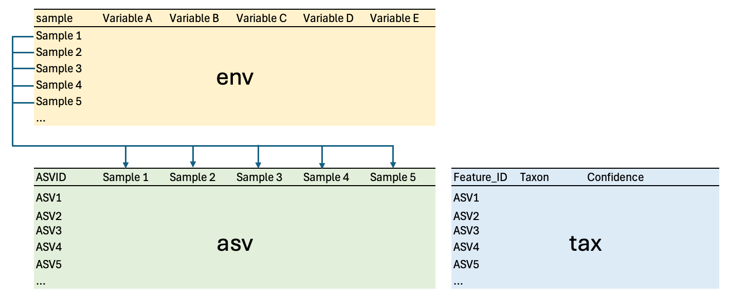
Relationships between tables

• asv and tax are related by the same hash (md5 checksum) key, but they are named ASVID in asv and Feature_ID in tax.
• asv and env are related based on column names in asv and sample column in env.

This is a graphical representation of their relationship with each other:

Joining tables using dplyr

To help us combine tabular data in R, we will use a set of *_join() functions from the dplyr package. Join functions can be used to add columns from one dataset to another dataset. If you are familiar with the relational database management system SQL, you should feel comfortable with these functions’ relational operations. These functions will return a NA for non-matching keys or missing observations while preserving valid joins for other observations.

Based on the previous lesson, we know that ammonia oxidisers often carry the "Nitroso-" prefix. The only table with that information is tax. To begin, we will subset that table to the relevant taxa and remove the Confidence metric.

code

amo <- filter(tax, str_detect(Taxon, "Nitroso")) %>%
  select(-Confidence)

We then need to add count per ASV per sample information from asv. To do this, we will use the left_join() function:

code

amo_abd <- left_join(amo, asv, by = join_by("Feature_ID" == "ASVID"))

Quite literally, the function joins the table on the right to the table on the left. We also use the by = argument and the join_by() function to specify which columns are keys in both tables. In layperson English, we can read the above as "join the asv table to the amo table where the columns Feature_ID in amo and ASVID in asv are keys".

The function left_join() is one of four mutating (sensu mutate() where new columns are appended to the table) joins in dplyr. The others are:

• right_join() Joins the table on the left to the table on the right (i.e., left_join() in the opposite direction).
• inner_join() Adds columns for matching keys in both tables.
• full_join() Adds columns for all keys in both tables.

Practical use

In my experience, left_join() is sufficient for most cases and is often the default choice for many users for its readable syntax (especially in chained pipes). However, there are some compelling cases for using inner_join() and full_join().

Many bioinformatics analyses are run in parallel (e.g., annotations against multiple databases or sequence curation using multiple software) to obtain as much information as possible about a given sequence. Essentially, these are identical sequences analysed in different ways.

Let’s assume that we are interested in well-characterised genes and pathways. Multiple analyses should produce concordant results for a subset of sequences thereby reducing the chance of false positives or hits with low probability of homology (e.g., a query sequence with homology to citrate synthase should be found regardless of searches against KEGG, NCBI RefSeq, or UniProt databases). In this scenario, using inner_join() will create a table that includes only those results that are consistent across analyses.

Under different circumstances we might be interested in looking at all the outputs captured by multiple analyses. For example when looking for novel or less well-characterised genes, suspect some analyses may propagate database biases, or want to perform further analyses to eliminate redundancies based on home-grown criteria. Here, we are likely more interested in preventing false negatives. In this case use full_join() to preserve all data points for further curation.

Cleaning up Taxon and summarising data

Next, lets use our skills from the previous lesson to only pick out "Nitroso-" from the Taxon column. Given that ggplot2 requires data in "long" format, we will also pivot the data and create sums of the abundance values so we have an overview of the distribution of ammonia oxidisers.

code

amo_summary <- amo_abd %>%
  mutate(
    Taxon = str_replace(Taxon, ".*(Nitroso[^;]+).*", "\\1")
  ) %>%
  pivot_longer(
    cols = where(is.numeric), 
    names_to = "sample", 
    values_to = "abundance"
  ) %>%
  group_by(sample, Taxon) %>%
  summarise(
    total = sum(abundance, na.rm = TRUE)
  )

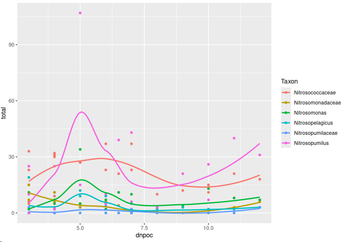
Joining environmental variables

Finally, we need to join environmental variables to our ammonia oxidiser abundance table. Then, we can plot the data using ggplot2.

code

amo_summary <- left_join(amo_summary, env, by = join_by("sample"))

# Plot using ggplot2
ggplot(amo_summary, aes(x = dnpoc, y = total, colour = Taxon)) +
  geom_point() +
  geom_smooth(method = "loess", se = F)

Duplicated keys

The keys in the asv table are MD5 hash values generated directly based on the sequence data. A benefit of using this convention is that adding more sequences to the analysis involves very little remapping of sequence to IDs. Thanks to the way MD5 hash algorithm works, read counts from the new batch will be added to read counts from the previous batch if they were the same ASV, while new unique sequences will be appended to the table as new entries.

However, what would happen if we tried to join data that had redundancies in their key naming conventions? In this case, the default behaviour of mutating joins is to output the Cartesian product of both data frames based on their keys. That is to say, all possible combinations of the keys will be used to generate the newly joined table.

(Optional) Filtering joins

dplyr also has two filtering joins (sensu filter() where rows are removed/retained based on keys). These are:

• anti_join() removes rows if keys in x match those in y.
• semi_join() retains rows if keys in x match those in y.

These are similar to piping a data frame to a filter():

code

# anti_join(x, y)
filter(x, key %in% y$key)

# semi_join(x, y)
filter(x, !(key %in% y$key))

Personally, I prefer using filter() for its flexibility and verbose syntax, and then perform joining operations when necessary.