Phylogenetic tree visualisation

Published

March 12, 2025

Load libraries

library(ggtree)

ggtree v3.14.0 Learn more at https://yulab-smu.top/contribution-tree-data/

Please cite:

Guangchuang Yu. Using ggtree to visualize data on tree-like structures.
Current Protocols in Bioinformatics. 2020, 69:e96. doi:10.1002/cpbi.96

library(phangorn)

Loading required package: ape


Attaching package: 'ape'

The following object is masked from 'package:ggtree':

    rotate

library(ggplot2)
library(ggtreeExtra)

ggtreeExtra v1.16.0 For help: https://yulab-smu.top/treedata-book/

If you use the ggtree package suite in published research, please cite
the appropriate paper(s):

S Xu, Z Dai, P Guo, X Fu, S Liu, L Zhou, W Tang, T Feng, M Chen, L
Zhan, T Wu, E Hu, Y Jiang, X Bo, G Yu. ggtreeExtra: Compact
visualization of richly annotated phylogenetic data. Molecular Biology
and Evolution. 2021, 38(9):4039-4042. doi: 10.1093/molbev/msab166

library(ape)
library(dplyr)


Attaching package: 'dplyr'

The following object is masked from 'package:ape':

    where

The following objects are masked from 'package:stats':

    filter, lag

The following objects are masked from 'package:base':

    intersect, setdiff, setequal, union

library(tidyr)


Attaching package: 'tidyr'

The following object is masked from 'package:ggtree':

    expand

Import Newick tree file generated by FastTree and created a tree object

tree <- read.tree("~/Desktop/GA2025/01.Short_read_workshop/SR_workshop/temp/tree_file.txt")

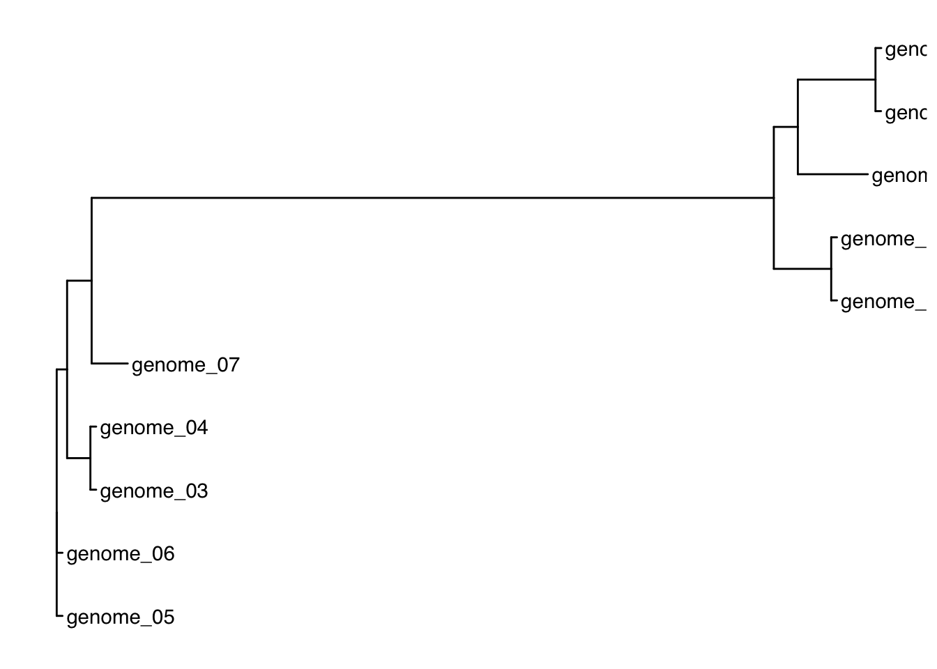
Now we can visualize the phylogenetic tree with ggtree

ggtree(tree) + geom_tiplab()

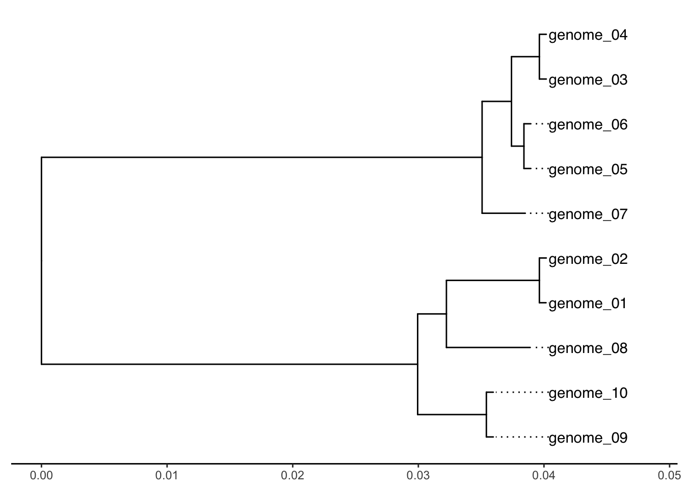
This quick and easy tree doesn’t include a reference genome, so we can use the midpoint() function of the phangorn package to reroot the tree at midpoint (i.e. locate the midpoint of the longest path between any two tips and place the root at that location, assuming a constant evolutionary rate).

#Rerooting tree at midpoint
reroot_tree <- midpoint(tree)

# Rescale tree based on the maximum tree depth and plot a cleaned up version of the tree
tree_depth <- max(node.depth.edgelength(reroot_tree))

p0 <-  ggtree(reroot_tree) + 
  geom_tiplab(align = TRUE, linesize = 0.5) +  
  xlim(0, tree_depth * 1.2) +
  theme_tree2()
p0

Let’s now visualise some of the genome quality metrics that were gathered during the workshop. Read in the genome metadata.

qual <- read.delim("~/Desktop/GA2025/01.Short_read_workshop/SR_workshop/temp/genome_quality.txt")

Join tree info with metadata.

# Generate random values for each tip label in the data
d1 <- data.frame(id=reroot_tree$tip.label)
colnames(d1)[1] <- "ID"
d1 <- left_join(d1, qual, "ID")

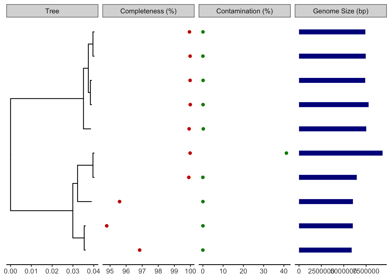
Facet plot for completeness, contamination, and genome size.

#Facet for tree
p1 <- ggtree(reroot_tree)
#Facet for genome completeness
p2 <- facet_plot(p1, panel="Completeness (%)", data=d1, geom=geom_point, aes(x=Completeness), color='red3')
#Facet for genome contamination
p3 <- facet_plot(p2, panel="Contamination (%)", data=d1, geom=geom_point, aes(x=Contamination), color='green4')
#Facet for genome size
p4 <- facet_plot(p3, panel="Genome Size (bp)", data=d1, geom=geom_segment, aes(x=0, xend=Genome_Size, y=y, yend=y), size=3, color='blue4')

# Show all three plots with a scale
p4 + theme_tree2()