Scaling-up Gene Regulatory Network Simulations

with an introduction to parallelisation and High Performance Computing

Olivia Angelin-Bonnet, New Zealand eScience Infrastructure

21-22 September 2022

1. Introduction

Why simulations are important in research

Model: mathematical or statistical representation of a system or phenomenon (cell, ecosystem, solar system, etc).
Simulation: Data about the system generated using a mathematical or statistical model.

Models and simulations allow us to:

Explain experimental data (through model fitting and refinement);
Test hypotheses:
- without going through expensive and time-consuming experiments;
- that wouldn’t be ethical or even feasible to test in real life.
Make predictions about new interventions/scenarios;
Communicate knowledge.

Modelling and simulations are used in many fields of science, e.g.:

Epidemiology: modelling of infectious diseases (see this talk on COVID-19 modelling);
Ecology: modelling of ecosystems, prediction of species abundance, evaluation of conservation policies;
Medicine: construction of organ models, prediction of drug-target binding and drug efficiency;
Chemistry, molecular biology: molecules interaction models;
Astrophysics: modelling of planet formation, galaxy mergers (see this example);
and many more!

Systems Biology: the study of the interactions between biological entities through modelling and simulations

Interdisciplinary field: builds on physics, chemistry, biology, computer science, statistics, mathematics, etc
Interest in understanding the emerging properties of biological systems arising from local interactions between molecular components
Construction of whole-cell computational model of the human pathogen Mycoplasma genitalium: Kar et al., Cell (2012)

What are Gene Regulatory Networks?

An overview of gene expression:

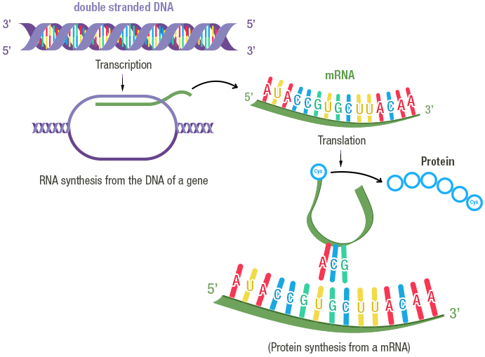
Credit: Fondation Merieux

Regulation of gene expression:

Cells adapt to changes in environment by modulating the expression of their genes
Gene expression regulated by different types of molecules:
- proteins
- regulatory non-coding RNAs
- small metabolites

Expression of a target gene can be controlled in different ways:

Regulation of transcription (regulatory proteins called transcription factors or TFs)
Regulation of translation
Regulation of gene products’ decay (RNAs and proteins)
Post-translational regulation (modification of sequence or shape of target proteins)

Note

Regulation that increases the target’s expression \(\rightarrow\) activation

Regulation that reduces/suppresses the target’s expression \(\rightarrow\) repression

A Gene Regulatory Network:

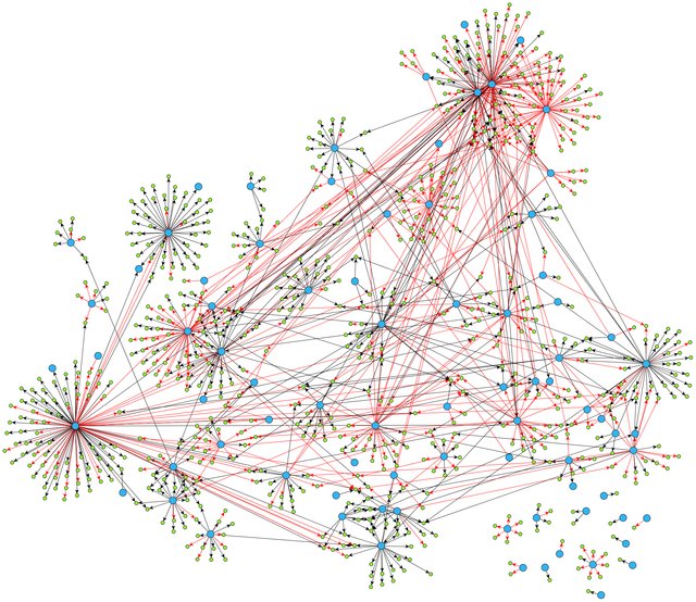
From Ma, Sisi, et al. “De-novo learning of genome-scale regulatory networks in S. cerevisiae.” Plos one 9.9 (2014): e106479. (available under license CC BY 4.0)

Not all genes linked to all others: relationship between regulator and target usually very specific:

most targets controlled only by a few regulators;
most regulators controlling only a few targets;
some “hub” or “master” regulators.

Simulating Gene Regulatory Networks

Why simulating GRNS?

to test hypotheses about the GRN (e.g. by comparing simulations to experimental data);
to predict the response to a specific condition;
to predict the response of the system to a modification of the GRN;
to understand the emerging properties of the system;
to evaluate the performance of statistical tools used for GRN reconstruction from gene expression data.

Building blocks of a GRN model:

A list of regulatory interactions between the genes (often represented as a graph);
A set of rules to convert the regulations into a mathematical or statistical model;
(optional, depends on the model): A set of numerical parameters specifying the rate of the different reactions in the model.

Note

There are many types of models that can be used to model GRNs!

Logical models

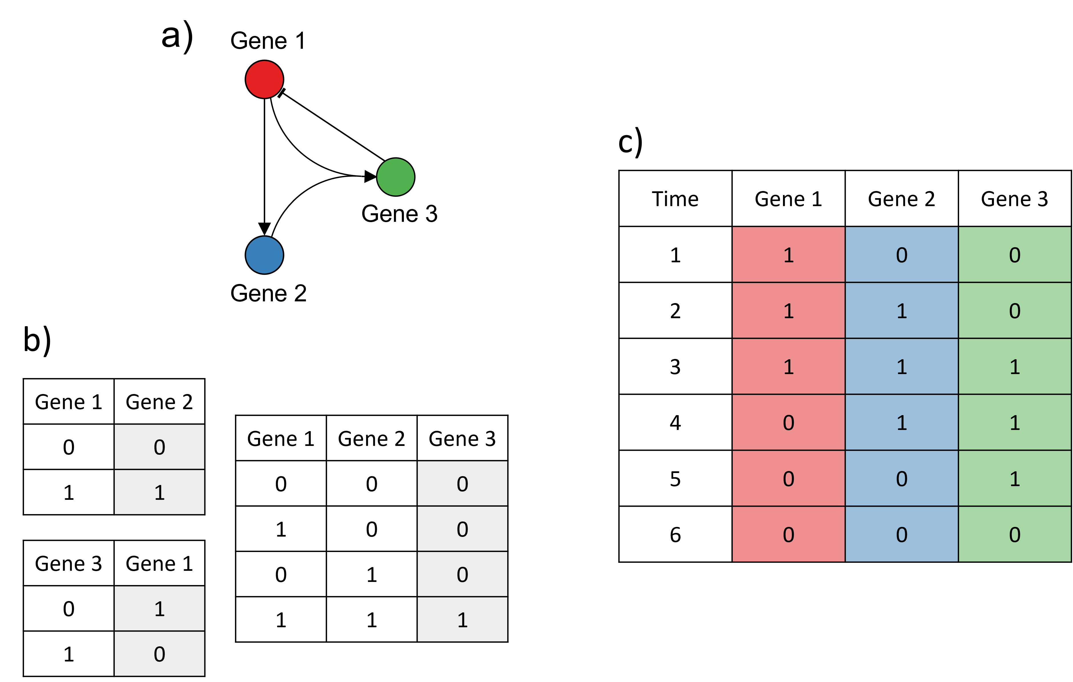
Example adapted from Karlebach, G., Shamir, R. Modelling and analysis of gene regulatory networks. Nat Rev Mol Cell Biol 9, 770--780 (2008). https://doi.org/10.1038/nrm2503.

Continuous and deterministic models

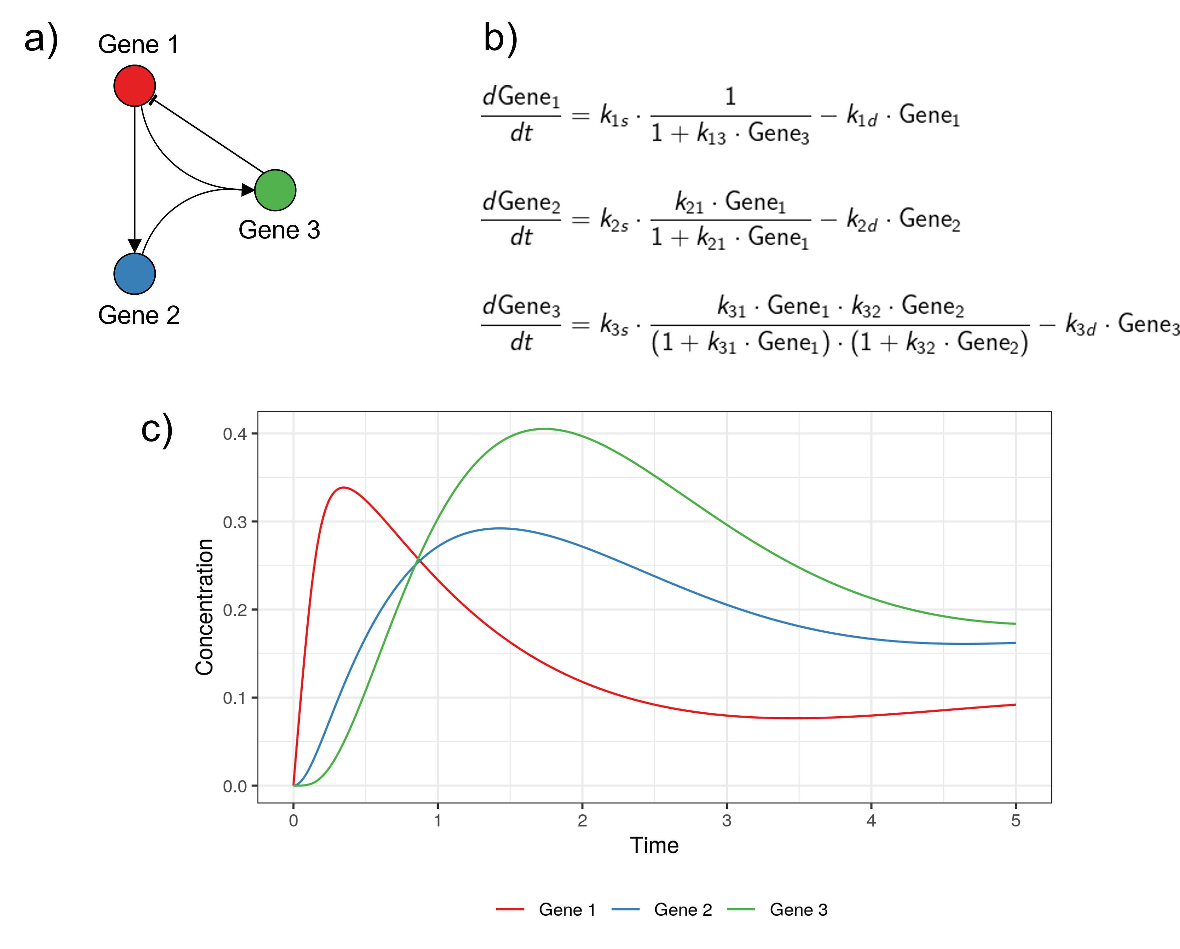
Example adapted from Karlebach, G., Shamir, R. Modelling and analysis of gene regulatory networks. Nat Rev Mol Cell Biol 9, 770--780 (2008). https://doi.org/10.1038/nrm2503.

Discrete and stochastic models

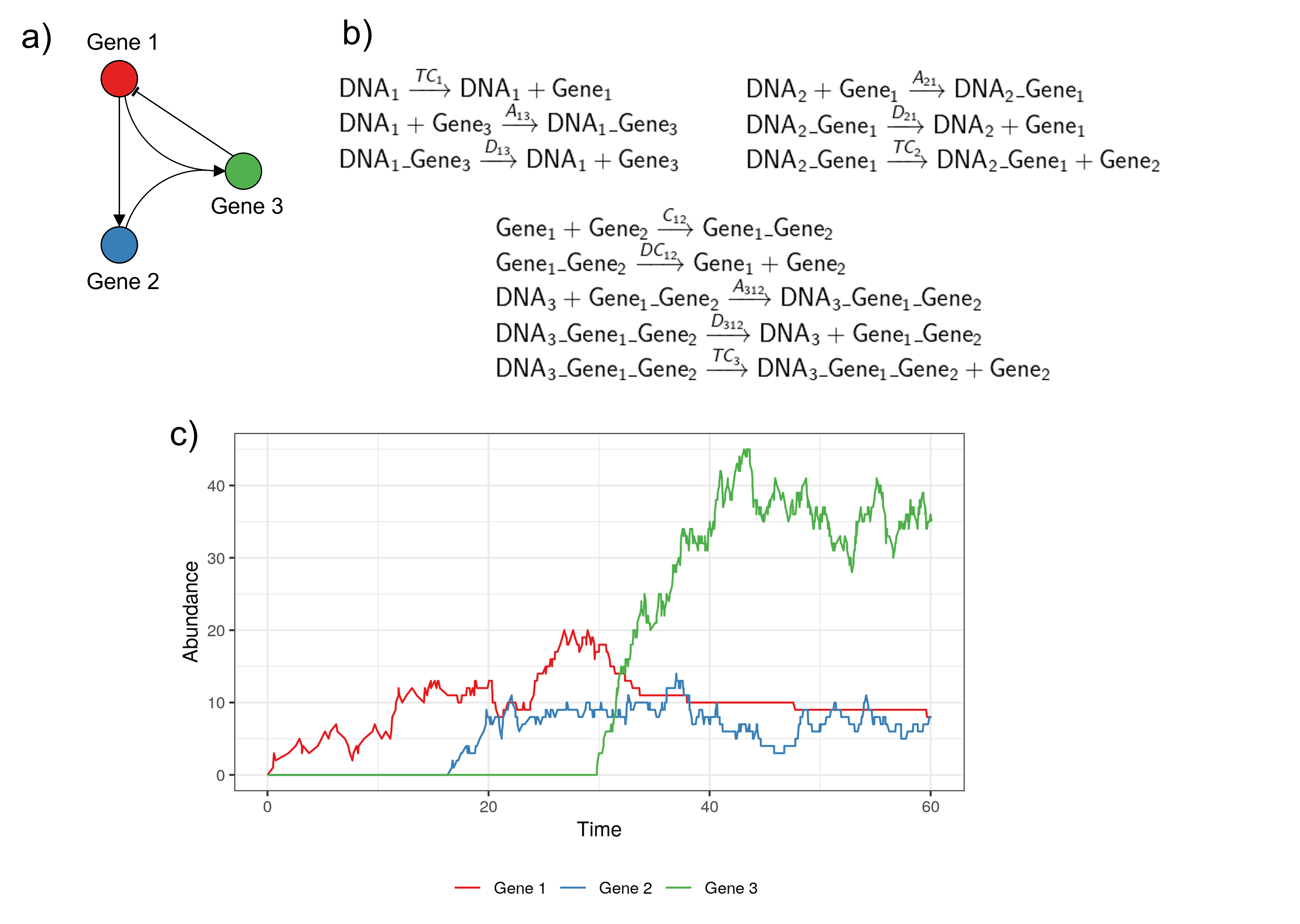
R code to reproduce the last two examples available here.

Each type of model has its own advantages and drawbacks:

Some tools available to simulate GRNs (not an exhaustive list!)

GeneNetWeaver: for deterministic or semi-stochastic modelling;
CaiNet: mix of probabilistic and deterministic equations;
MeSCoT: stochastic modelling with time-delay;

sismonr: R package for stochastic modelling.

In this workshop, we’ll focus on discrete and stochastic models:

good option to simulate species (i.e. molecules) with very low abundance per cell (e.g. transcription factors);
but computationally heavy, which restricts the size of the models that can be simulated.

A brief introduction to the Stochastic Simulation Algorithm

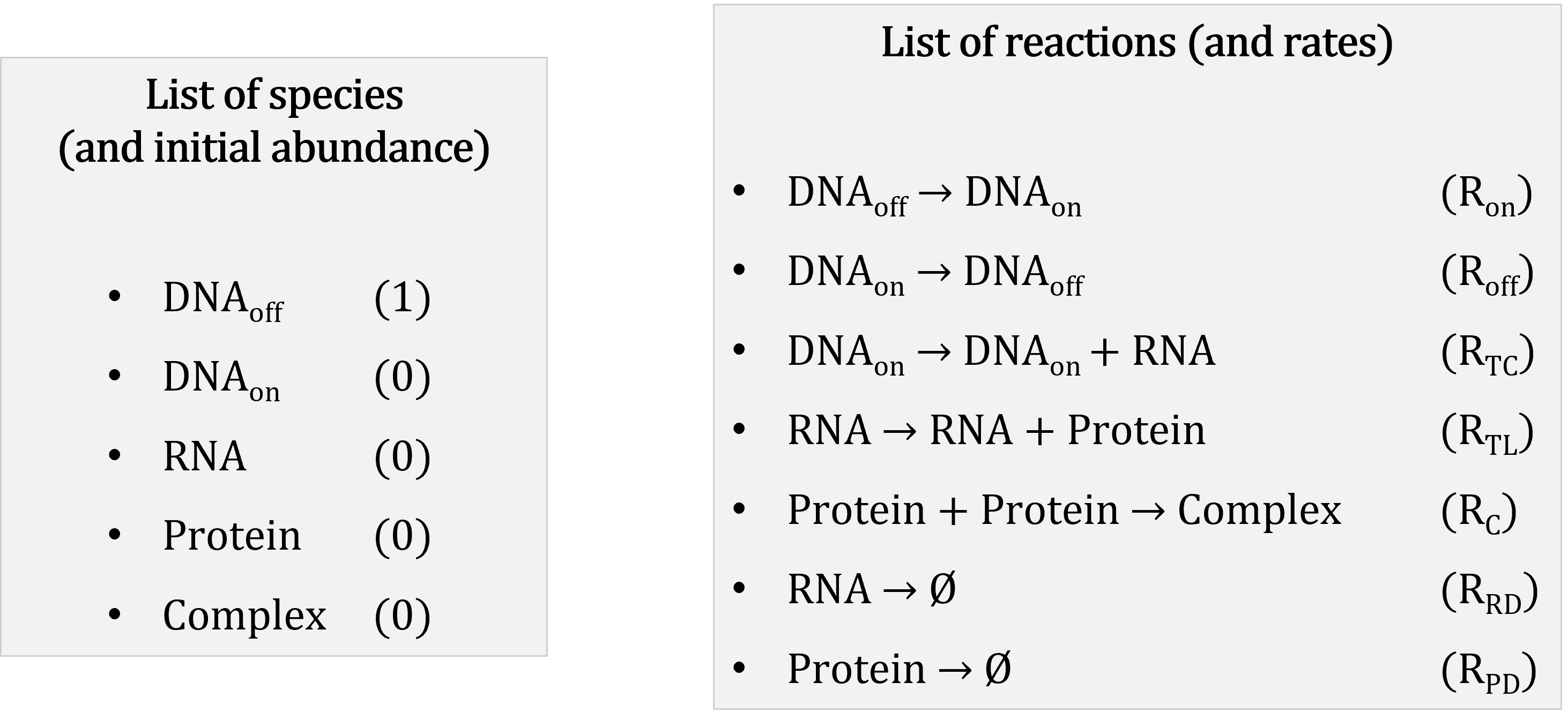
A stochastic model consists of:

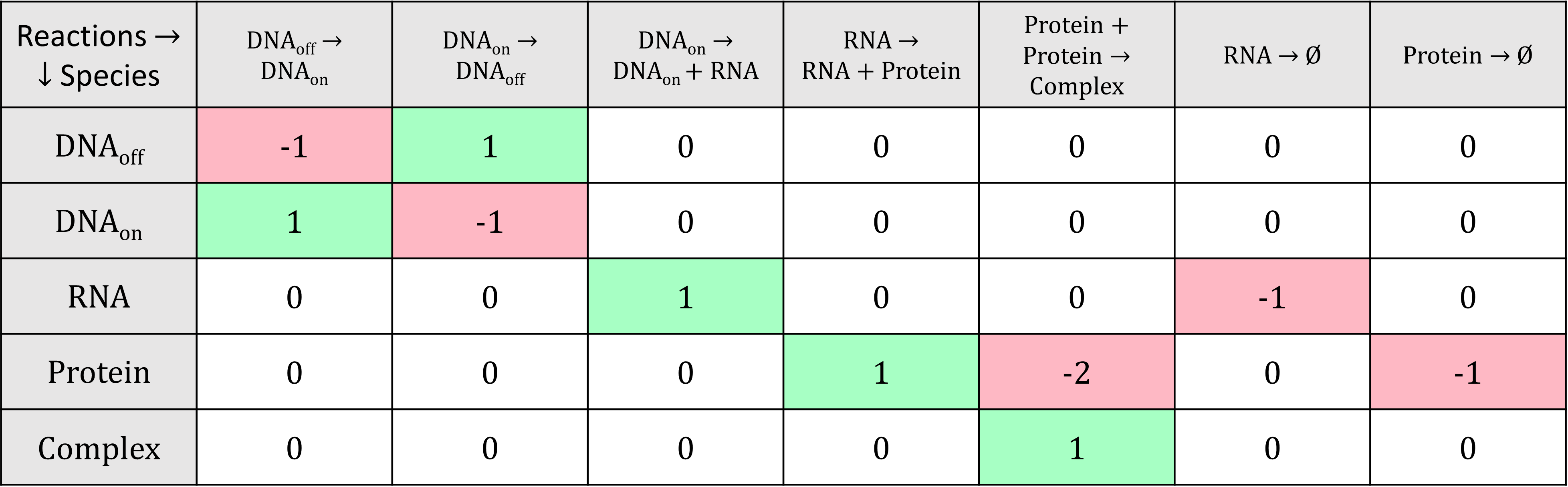
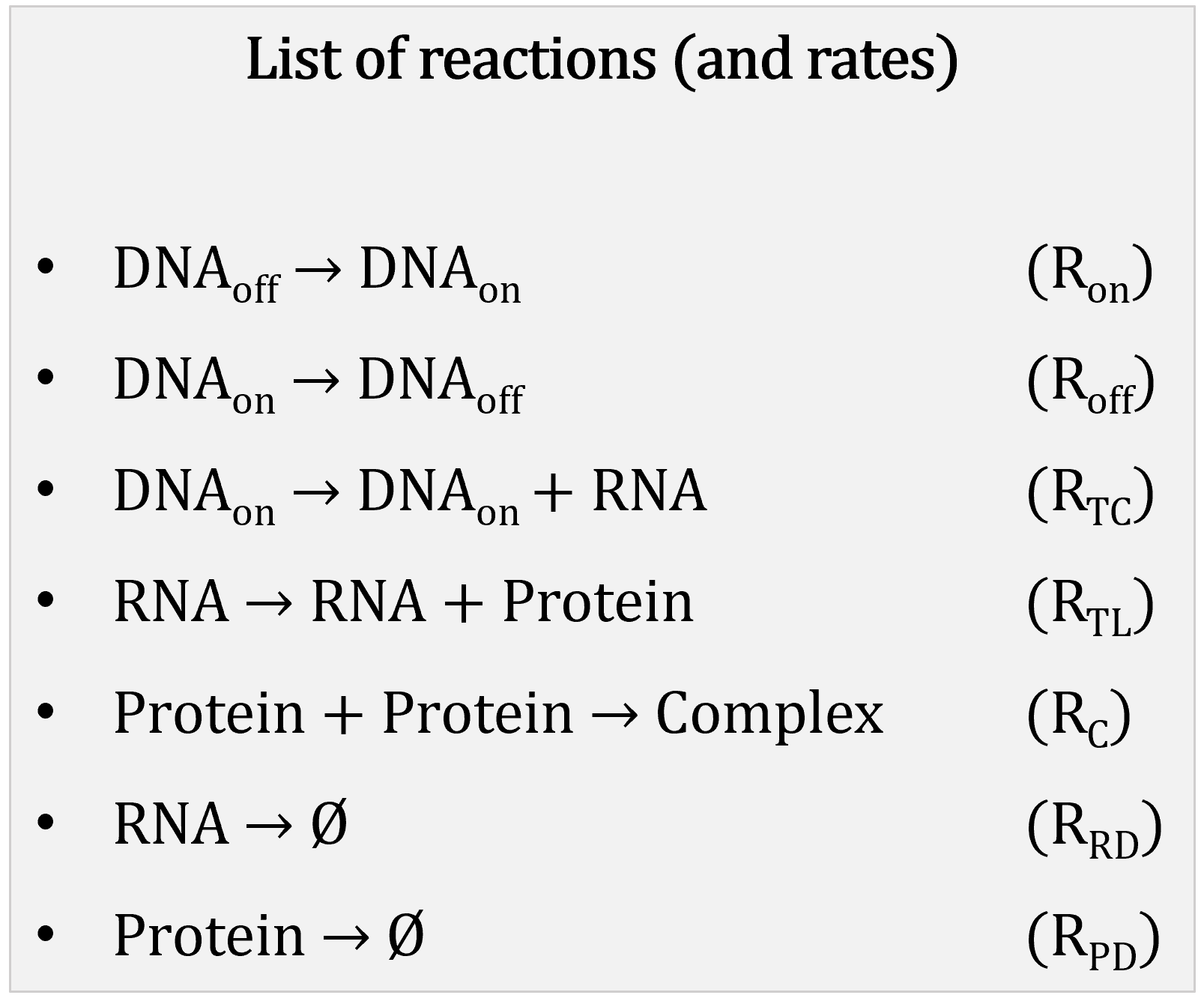
Reactions represented with a stoichiometry matrix:

System state represented as vector of species abundance at a given time point:

To simulate the evolution of the system over time, we need to know which reaction will fire when.

Reaction propensity: probability of the reaction to occur in the next (small) unit time step

Propensity depends on:

constant rate of the reaction
state of the system at a current time point:
- few reactants present in the system \(\rightarrow\) low chance of the reaction occurring;
- reactants abundant in the system: \(\rightarrow\) high chance of the reaction occurring.

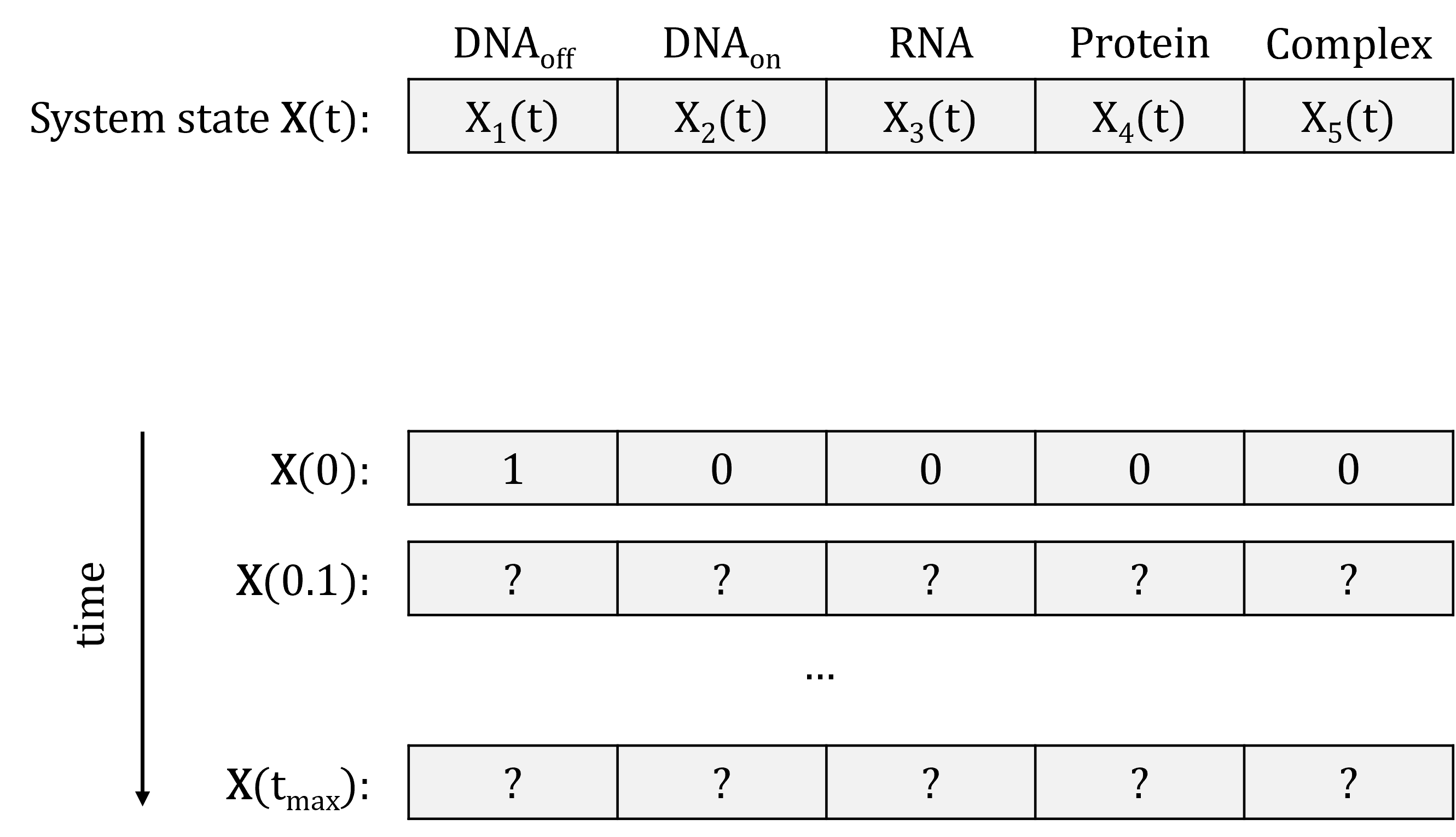
In our example:

Basic concept of the Stochastic Simulation Algorithm:

Initialisation: set \(t = 0\), and initial system state as initial species abundance.

Compute reactions propensities, based on current system state.
Randomly generate time increment \(\tau\) during which next reaction occurs.
Randomly select which reaction will occur between \(t\) and \(t+ \tau\).
Update time to \(t + \tau\) and system state based on which reaction occurred.
Repeat steps 1 to 4, until \(t = t_{max}\).

An example of one SSA iteration:

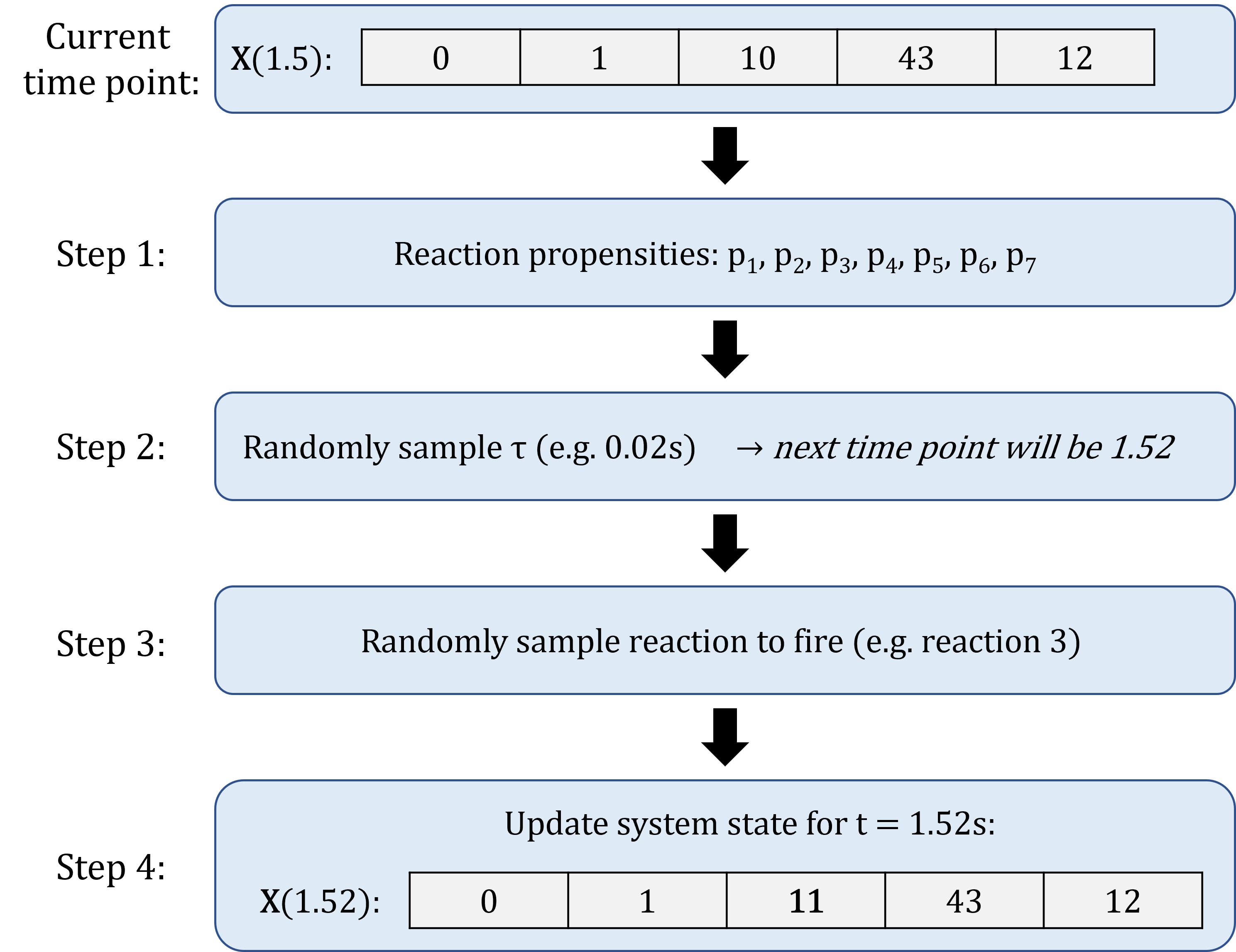
Advantage of SSA: every single reaction is simulated!

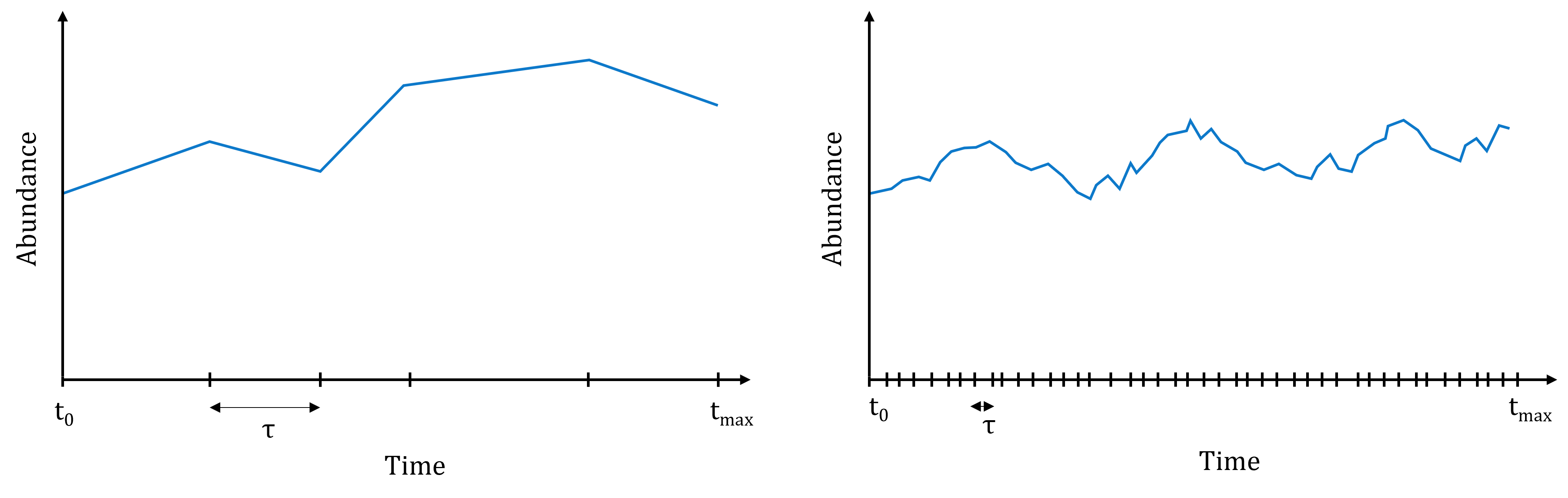
Downside: if many reactions with high propensity, each time increment will be really small

\(\rightarrow\) will take a long time to get to the end of the simulation

There exist many variations of the SSA:

exact versions: simulate the occurrence of every single reaction;
approximate versions: trade-off between accuracy and computational burden.

Several implementations of the SSA:

R: GillespieSSA, adaptivetau
python: gillespie
Julia: BioSimulator.jl – used by the sismonr package that we are going to use!

2. Getting started with sismonr

Introduction to the sismonr package

sismonr was developed for the purpose of generating benchmark datasets to assess the performance of network reconstruction methods

Objectives:

include the effect of small genetic mutations in the GRN to mimic genetic variability between individuals;
allow the simulation of polyploid systems (i.e. more that 2 copies of each gene present in the system);
model post-transcriptional regulation;
transparent model, customisable by the user;
generate random but plausible GRNs or use GRN provided by user.

Note

A complete sismonr tutorial is available here.

can be slow for intensite computations \(\rightarrow\) sismonr uses under the hood!

sismonr uses the XRJulia package to link R and Julia:

Socket connection initialised on a random port \(\rightarrow\) can get messy when working on a HPC…

Solution:

XRJulia::newJuliaEvaluator(port = as.integer(456))

Some sismonr abbreviations:

Abbreviations	Meaning
TC	Transcription
TL	Translation
RD	RNA decay
PD	Protein decay
PTM	Post-translational modification
PC	Protein-coding
NC	Noncoding
R	RNA
P	Protein
Pm	Modified protein
C	Regulatory complex

Practice time!

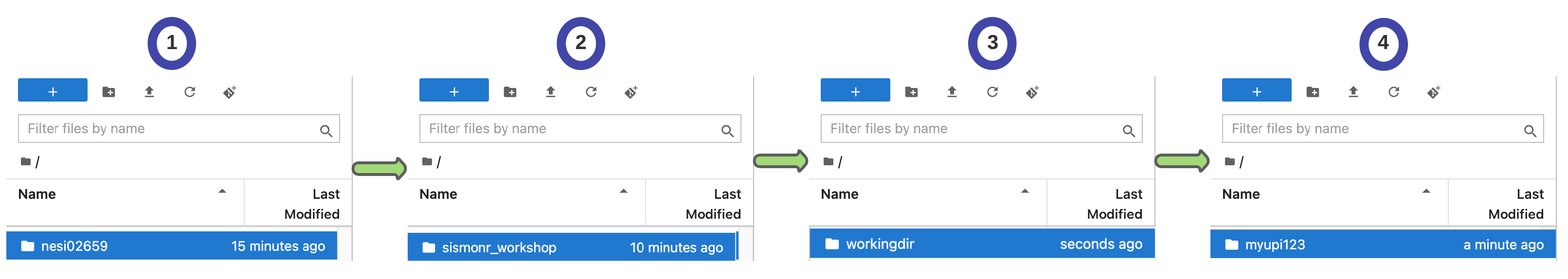
Instructions to log in to NeSI Mahuika Jupyter in the Supplementary Material.

Important

Do not forget to change your working directory!