Over-representation analysis (Gene Ontology)
Objectives
- Identify enriched biological functions or processes within a list of differentially expressed genes
- Recognise the importance of gene length in over-representation analyses, and how to correct for this in your analysis
- Slides: lecture_annotation_pathways.pdf
Over-representation Analysis (Boyle et al. 2004) is a widely used approach to determine whether known biological functions or processes are over-represented (= enriched) in an experimentally-derived gene list, e.g. a list of differentially expressed genes (DEGs).
- Can perform over-representation analysis online (e.g., Enrichr, GeneSetDB, PantherDB), and also in R.
- The basic principles are to:
- identify a collection of differentially expressed genes
- test to see if genes that are members of specific gene sets (e.g., Reactome pathways, Gene Ontology categories) are differentially expressed more often than would be expected by chance.
Some caveats for RNA-seq data
- The gene-set analysis methods are applicable to transcriptomic data from both microarrays and RNA-seq.
- One caveat, however, is that the results need to take gene length into account.
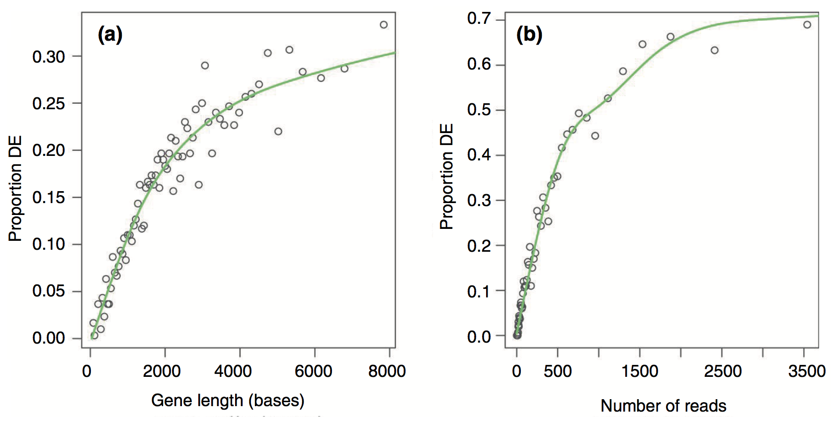
- RNA-seq tends to produce higher expression levels (i.e., greater counts) for longer genes: a longer transcript implies more aligned fragments, and thus higher counts. This also gives these genes a great chance of being statistically differentially expressed.
- Some gene sets (pathways, GO terms) tend to involve families of long genes: if long genes have a great chance of being detected as differentially expressed, then gene sets consisting of long genes will have a great chance of appeared to be enriched in the analysis.
GOseq
- The GOseq methodology (Young et al., 2010) overcomes this issue by allowing the over-representation analysis to be adjusted for gene length.
- modification to hypergeometric sampling probability
- exact method (resampling) and an approximation-based method
- More recent publications have also applied this gene-length correction to GSEA-based methods.
- Still not widely understood to be an issue when performing RNA-seq pathway analysis, but REALLY important to take into account.
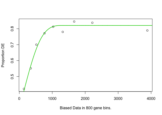
Results from the Young et al (2010) publication:
GOseq analysis
Need to figure out if our organism is supported… (code is “sacCer”)
##          Genome         Id  Id Description Lengths in geneLeneDataBase
## 10      anoCar1    ensGene Ensembl gene ID                        TRUE
## 11      anoGam1    ensGene Ensembl gene ID                        TRUE
## 132     anoGam3                                                  FALSE
## 12      apiMel2    ensGene Ensembl gene ID                        TRUE
## 137 Arabidopsis                                                  FALSE
## 56      bosTau2 geneSymbol     Gene Symbol                        TRUE
##     GO Annotation Available
## 10                    FALSE
## 11                     TRUE
## 132                    TRUE
## 12                    FALSE
## 137                    TRUE
## 56                     TRUE
Easier to find if we use View() (NB - this only works in RStudio. Can’t use if working in a Jupyter Notebook).
Define differentially expressed genes
- Create a vector of 0’s and 1’s to denote whether or not genes are differentially expressed (limma analysis: topTable).
- Add gene names to the vector so that GOSeq knows which gene each data point relates to.
Load our topTable results from last session:
# Note: If you want to use tt from DESeq, replace $adj.P.Val with $padj below

genes = ifelse(tt$adj.P.Val < 0.05, 1, 0)
names(genes) = rownames(tt)
head(genes)
## YAL038W YOR161C YML128C YMR105C YHL021C YDR516C
##       1       1       1       1       1       1
## genes
##    0    1
## 1987 5140
Calculate gene weights
- Put genes into length-based “bins”, and plot length vs proportion differentially expressed
- Likely restricts to only those genes with GO annotation
Inspect output
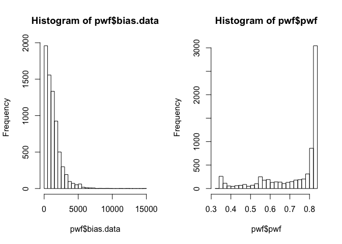
Report length (bias) and weight data per gene.
##         DEgenes bias.data       pwf
## YAL038W       1      1504 0.8205505
## YOR161C       1      1621 0.8205505
## YML128C       1      1543 0.8205505
## YMR105C       1      1711 0.8205505
## YHL021C       1      1399 0.8205505
## YDR516C       1      1504 0.8205505
Gene lengths and weights
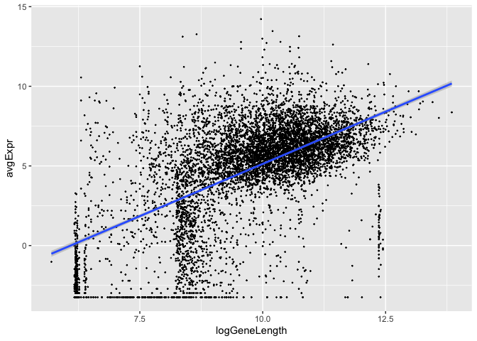
Gene length vs average expression
Is there an association between gene length and expression level?
library(ggplot2)
data.frame(logGeneLength = log2(pwf$bias.data),
           avgExpr = tt$AveExpr) %>%
  ggplot(., aes(x=logGeneLength, y=avgExpr)) +
  geom_point(size=0.2) +
  geom_smooth(method='lm')
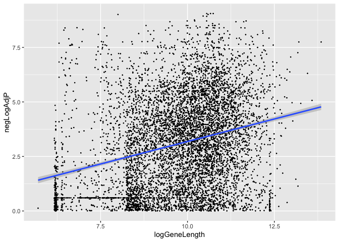
How about gene length and statistical evidence supporting differential expression?
(Kinda hard to see, but it is apparently there…)
data.frame(logGeneLength = log2(pwf$bias.data),
           negLogAdjP = -log10(tt$adj.P.Val)) %>%
  ggplot(., aes(x=logGeneLength, negLogAdjP)) +
  geom_point(size=0.2) +
  geom_smooth(method='lm')
Length correction in GOSeq
- Uses “Wallenius approximation” to perform correction.
- Essentially it is performing a weighted Fisher’s Exact Test, but each gene in the 2x2 data does not contribute equally to the per cell count - it instead contributes its weight (based on its length).
- This means that a gene set (e.g., GO term) containing lots of significant short genes will be considered more likely to be enriched that a gene set with a similar proportion of long genes that are differentially expressed.
Run GOSeq with gene length correction:
Output: Wallenius method
##        category over_represented_pvalue under_represented_pvalue numDEInCat
## 1325 GO:0005622            1.817597e-17                        1       4298
## 7912 GO:0110165            8.200109e-12                        1       4456
## 5245 GO:0042254            9.441146e-12                        1        364
## 3817 GO:0022613            1.355385e-11                        1        439
## 5446 GO:0043226            2.516156e-11                        1       3826
## 5449 GO:0043229            4.433252e-11                        1       3817
##      numInCat                                 term ontology
## 1325     5179                        intracellular       CC
## 7912     5417           cellular anatomical entity       CC
## 5245      395                  ribosome biogenesis       BP
## 3817      482 ribonucleoprotein complex biogenesis       BP
## 5446     4609                            organelle       CC
## 5449     4599              intracellular organelle       CC
P-value adjustment
## [1] 45
## [1] 45
## [1] "GO:0005622" "GO:0110165" "GO:0042254" "GO:0022613" "GO:0043226"
## [6] "GO:0043229"
Filtering by gene set length
We are usually not interested in pathways or ontology terms that involve large numbers of genes (they are often rather broad terms or mechanisms), so we can exclude these from the results (here we only include significant GO terms that involve less than 500 genes):
Output
##      category over_represented_pvalue under_represented_pvalue numDEInCat
## 1  GO:0042254            9.441146e-12                1.0000000        364
## 2  GO:0022613            1.355385e-11                1.0000000        439
## 3  GO:0030684            3.348423e-08                1.0000000        163
## 4  GO:0016072            3.873737e-08                1.0000000        274
## 5  GO:0006364            4.532117e-08                1.0000000        259
## 6  GO:0034470            2.776978e-07                1.0000000        360
## 7  GO:0030490            9.891093e-07                0.9999998        111
## 8  GO:0030687            1.502461e-06                1.0000000         62
## 9  GO:0042274            2.616777e-06                0.9999993        134
## 10 GO:0005730            3.753501e-06                1.0000000        264
## 11 GO:0003735            3.799990e-06                1.0000000        194
## 12 GO:0022626            4.824970e-06                0.9999984        140
## 13 GO:0044391            6.732064e-06                1.0000000        202
## 14 GO:0000462            1.221128e-05                0.9999977         99
## 15 GO:0005840            1.780243e-05                0.9999942        221
## 16 GO:0002181            2.156069e-05                0.9999913        169
## 17 GO:0034660            7.782098e-05                0.9999571        409
## 18 GO:0042273            8.604282e-05                0.9999745        117
##    numInCat
## 1       395
## 2       482
## 3       171
## 4       299
## 5       282
## 6       401
## 7       116
## 8        62
## 9       143
## 10      292
## 11      221
## 12      156
## 13      231
## 14      104
## 15      254
## 16      191
## 17      467
## 18      126
##                                                                                        term
## 1                                                                       ribosome biogenesis
## 2                                                      ribonucleoprotein complex biogenesis
## 3                                                                               preribosome
## 4                                                                    rRNA metabolic process
## 5                                                                           rRNA processing
## 6                                                                          ncRNA processing
## 7                                                                    maturation of SSU-rRNA
## 8                                                      preribosome, large subunit precursor
## 9                                                        ribosomal small subunit biogenesis
## 10                                                                                nucleolus
## 11                                                       structural constituent of ribosome
## 12                                                                       cytosolic ribosome
## 13                                                                        ribosomal subunit
## 14 maturation of SSU-rRNA from tricistronic rRNA transcript (SSU-rRNA, 5.8S rRNA, LSU-rRNA)
## 15                                                                                 ribosome
## 16                                                                  cytoplasmic translation
## 17                                                                  ncRNA metabolic process
## 18                                                       ribosomal large subunit biogenesis
##    ontology
## 1        BP
## 2        BP
## 3        CC
## 4        BP
## 5        BP
## 6        BP
## 7        BP
## 8        CC
## 9        BP
## 10       CC
## 11       MF
## 12       CC
## 13       CC
## 14       BP
## 15       CC
## 16       BP
## 17       BP
## 18       BP
GO terms
- Can use the
GO.dbpackage to get more information about the significant gene sets.
## GOID: GO:0005622
## Term: intracellular
## Ontology: CC
## Definition: The living contents of a cell; the matter contained within
##     (but not including) the plasma membrane, usually taken to exclude
##     large vacuoles and masses of secretory or ingested material. In
##     eukaryotes it includes the nucleus and cytoplasm.
## Synonym: internal to cell
## Synonym: protoplasm
## Synonym: nucleocytoplasm
## Synonym: protoplast
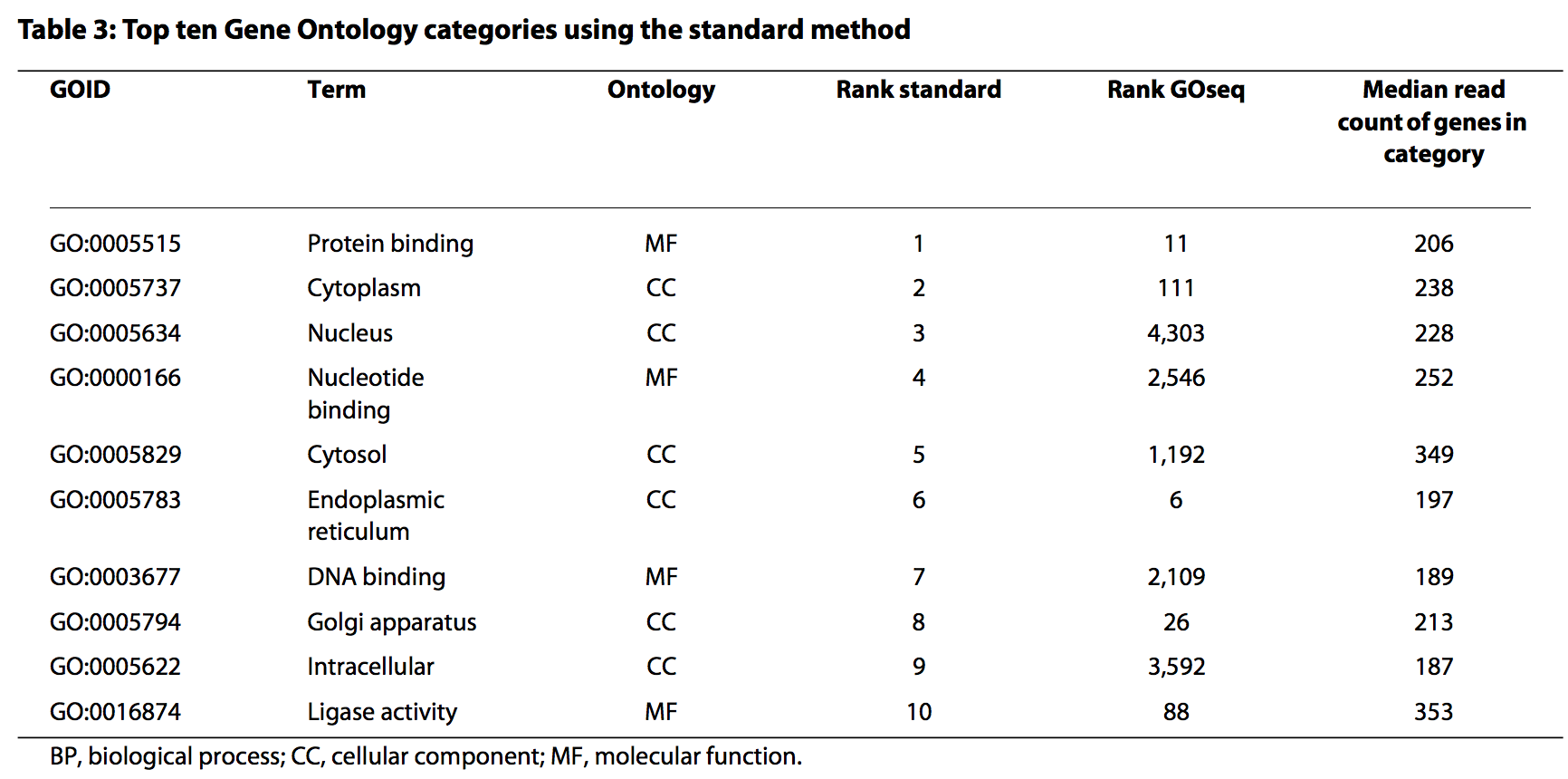
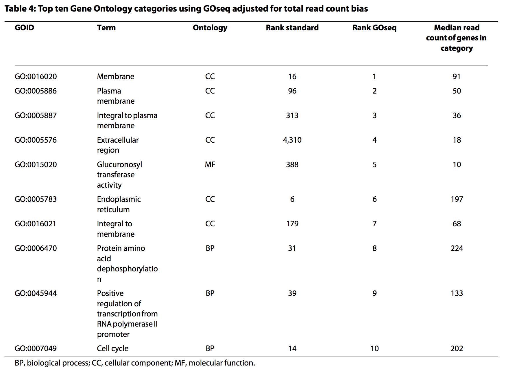
NB - the code below is demonstrating the difference between running with and without the gene length correction that GOseq implements. You wouldn’t usually work through this as part of a standard pathway analysis.
Run GOSeq without gene length correction
Output: Hypergeomtric (Fisher) method
##        category over_represented_pvalue under_represented_pvalue numDEInCat
## 1325 GO:0005622            8.650971e-29                        1       4298
## 7912 GO:0110165            3.271100e-21                        1       4456
## 5446 GO:0043226            9.826546e-16                        1       3826
## 2650 GO:0009987            1.330459e-15                        1       4146
## 5449 GO:0043229            2.060920e-15                        1       3817
## 5245 GO:0042254            7.222008e-11                        1        364
##      numInCat                       term ontology
## 1325     5179              intracellular       CC
## 7912     5417 cellular anatomical entity       CC
## 5446     4609                  organelle       CC
## 2650     5023           cellular process       BP
## 5449     4599    intracellular organelle       CC
## 5245      395        ribosome biogenesis       BP
P-value adjustment
GO.nobias.padj = p.adjust(GO.nobias$over_represented_pvalue, method="fdr")
sum(GO.nobias.padj < 0.05)
## [1] 44
## [1] 44
## [1] "GO:0005622" "GO:0110165" "GO:0043226" "GO:0009987" "GO:0043229"
## [6] "GO:0042254"
Compare with and without adjustment
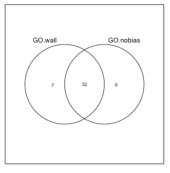
Extract out the different parts of the Venn diagram (yes, there are definitely better ways to do this).
## Only significant in Hypergeomtric analysis
onlySig.nobias = setdiff(GO.nobias.sig, GO.wall.sig)

## Only significant in Wallenius analysis
onlySig.wall = setdiff(GO.wall.sig, GO.nobias.sig)

## Significant in both
sig.wall.nobias = intersect(GO.wall.sig, GO.nobias.sig)
Gene lengths and GO term membership
Can also extract gene length and GO membership information.
## [1] 1504 1621 1543 1711 1399 1504
## [1] "YAL038W" "YOR161C" "YML128C" "YMR105C" "YHL021C" "YDR516C"
## [1] "list"
## [1] "GO:0006082" "GO:0008150" "GO:0008152" "GO:0009987" "GO:0019752"
## [6] "GO:0032787"
## [1] "GO:0006810" "GO:0008150" "GO:0009987" "GO:0051179" "GO:0051234"
## [6] "GO:0055085"
Getting fancy…
Figure out which genes are in the significant GO groups, and then gets their lengths.
lengths.onlySig.nobias = list()

for(i in 1:length(onlySig.nobias)){
  inGo = lapply(go, function(x)  onlySig.nobias[i] %in% x) %>% unlist()
  lengths.onlySig.nobias[[i]] = len[inGo]
}

lengths.onlySig.wall = list()

for(i in 1:length(onlySig.wall)){
  inGo = lapply(go, function(x)  onlySig.wall[i] %in% x) %>% unlist()
  lengths.onlySig.wall[[i]] = len[inGo]
}
Significant: Hypergeometric vs Wallenius
- Only Hypergeometric (pink) vs only Wallenius (blue)
- Hypergeometric method is findings GO terms containing longer genes.
cols = rep(c("lightpink", "lightblue"), c(10,7))
boxplot(c(lengths.onlySig.nobias, lengths.onlySig.wall), col=cols)
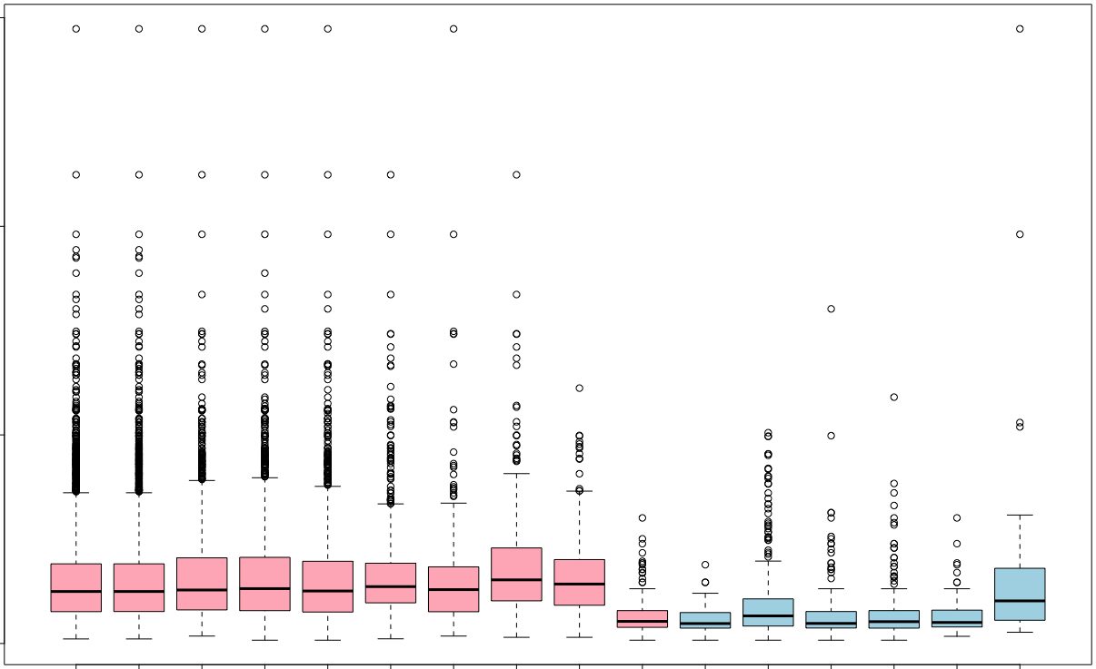
All significant GO terms
lengths.sig.wall.nobias = list()

for(i in 1:length(sig.wall.nobias)){
  inGo = lapply(go, function(x)  sig.wall.nobias[i] %in% x) %>% unlist()
  lengths.sig.wall.nobias[[i]] = len[inGo]
}
cols = rep(c("lightpink", grey(0.7), "lightblue"), c(10,37,7))

avgLength = lapply(c(lengths.onlySig.nobias, lengths.sig.wall.nobias, lengths.onlySig.wall),
                    median) %>% unlist()

oo = order(avgLength, decreasing=TRUE)
boxplot(c(lengths.onlySig.nobias, lengths.sig.wall.nobias, lengths.onlySig.wall)[oo],
        col=cols[oo], ylab="Gene Length", xlab = "GO term")
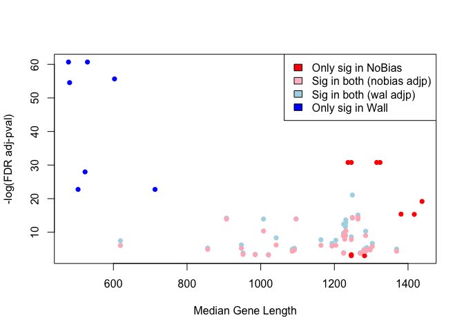
Gene length versus P-value
avgLength.wall = lapply(c(lengths.onlySig.wall, lengths.sig.wall.nobias), median)

avgLength.nobias = lapply(c(lengths.onlySig.nobias, lengths.sig.wall.nobias), median)

cols = rep(c("blue", "lightblue", "red","lightpink"),
            c(length(lengths.onlySig.wall), length(lengths.sig.wall.nobias),
              length(lengths.onlySig.nobias), length(lengths.sig.wall.nobias)))

plot(c(avgLength.wall, avgLength.nobias),
     -log(c(GO.nobias.padj[GO.nobias.padj < 0.05], GO.wall.padj[GO.wall.padj < 0.05])),
     col=cols, pch=16, xlab="Median Gene Length", ylab ="-log(FDR adj-pval)")
legend('topright', c("Only sig in NoBias", "Sig in both (nobias adjp)",
                     "Sig in both (wal adjp)", "Only sig in Wall"),
       fill=c("red", "pink", "lightblue", "blue"))
Summary
- Once we’ve generated count data, there are a number of ways to perform a differential expression analysis.
- DESeq2 and edgeR model the count data, and assume a Negative Binomial distribution
- Limma transforms (and logs) the data and assumes normality
- Here we’ve seen that these three approaches give quite similar results.
- For Gene Set analysis, gene length needs to be accounted for, since longer transcripts are more likely to be found to be differentially expressed.
- GOSeq adjusts for transcript length to take this into account.
- It is also possible to use GOSeq with other types of annotation (e.g., Reactome or KEGG pathways).