Tutorial¶

Aim

Go through the pipeline of phasing and imputing high-density genotype to sequence level
Understand the importance of quality control
Know how to evaluate the imputation performance

Import Notes

All the parameter settings are suggestive. A different population may get absolutely different results using the same setting.
You can't avoid experiments to find optimal settings for your own population before you started your whole genome sequence imputation.
Beagle 5.4 and Minimac3 are shown as examples in this tutorial. You can test on other software based on your need.

Tools we need

BCFtools: basic bioinformatics software, in this tutorial, we use it for creating subsets and quality control. The latest version is 1.17 but we will be using 1.16. (http://samtools.github.io/bcftools/bcftools.html)

VCFtools: basic bioinformatics software, in this tutorial, we use it for comparing two vcf files and evaluate the concordance rate. The current version on NeSI is 0.1.15 (https://vcftools.github.io/index.html)

R: basic statistics and plotting software

Beagle: software for phasing and imputation. The current version is beagle 5.4 (version: 22Jul22.46e). (https://faculty.washington.edu/browning/beagle/beagle.html) The performance of different versions of beagle can be found here: https://www.g3journal.org/content/10/1/177

Minimac3: software for imputation (https://genome.sph.umich.edu/wiki/Minimac3) Minimac has been updated to Minimac4 (https://github.com/statgen/Minimac4) but usage requires a file format change that is done with Minimac3

Input files

In this tutorial, we used 5MB segment (30-35MB) of chr13 from the 1000 Genome phase 3, which is publicly available and can be downloaded from https://mathgen.stats.ox.ac.uk/impute/impute_v2.html

Procedures¶

1. Load the modules that are required on NeSI¶

To find modules that are already available on NeSI module spider <module_name>
To load modules module load <module_name>

Open a terminal and at the prompt:

code

module purge
module load BCFtools/1.16-GCC-11.3.0
module load VCFtools/0.1.15-GCC-9.2.0-Perl-5.30.1
module load R/4.2.1-gimkl-2022a
module load Beagle/5.4-22Jul22.46e 
module load Minimac3/2.0.1

2. Copy the files into the home directory¶

Define two directories: workshop directory and home directory. In this workshop, the analysis will be conducted in your /home/$USER/imputation_workshop/ directory, (~ is the shortcut for you home directory)

code

cd ~
mkdir -p imputation_workshop
cd ~/imputation_workshop

The main input file (seqvcf) is extracted (from 30MB to 35MB) on chr13 from 1000 human genome data. I selected some of the reliable SNPs to generate a HD genotype dataset(hdvcf).

code

maindir=/nesi/project/nesi02659/imputation2021
seqvcf=$maindir/nonfilter_seq_5MB.vcf.gz
hdvcf=$maindir/hd_5MB.vcf.gz

Now what you need to do is to cp (copy) both the genotype and sequence data to your own home directory.

code

cp $seqvcf ~/imputation_workshop
cp $hdvcf ~/imputation_workshop

The genotype and sequence files use "vcf.gz" format. We can not open these compressed files directly. To check how the genotypes look, you need to use: zless -S. -S is to make the file well formatted and stops each line from wrapping around.

code

zless -S $seqvcf
zless -S $hdvcf

3. Explore the input file¶

When you got the dataset, the most important informaiton you may want to know is : 1. How many samples are there in my dataset 2. How many variants are there and where are they in my dataset

To have a basic idea of the genotype, BCFtools have a very convenient function to extract this information (https://samtools.github.io/bcftools/howtos/query.html)

code

bcftools query -l nonfilter_seq_5MB.vcf.gz | head 
bcftools query -l nonfilter_seq_5MB.vcf.gz | wc

bcftools query -f '%CHROM\t%POS\n' nonfilter_seq_5MB.vcf.gz | head 
bcftools query -f '%CHROM\t%POS\n' nonfilter_seq_5MB.vcf.gz | wc

If you want to have a deeper understanding of the dataset, like the number of SNPs, the number of indels, sequence depth etc, BCFtools have a very convenient function: stats. By checking the original sequence file's information. the code you need is as below. -s is a common tag to show "samples". Samples to include or "-" to apply all variants. Via adding this, we also generate the statistics for each individual. The output will be named: original.stats

code

bcftools stats -s "-" nonfilter_seq_5MB.vcf.gz > original.stats

Now let's have a look at the output:

code

less original.stats`

Output

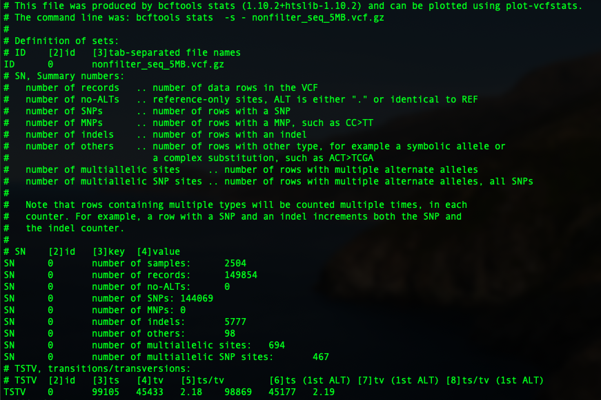
So in the first part, you can see the basic statistics of the sequence file. We have 2504 samples in total, with 149,854 variants. 144,069 of them are SNPs, 5777 indels, 98 other, 694 multi-allelic sites with 467 multi-allelic SNPs.

4. Quality control process¶

There are a lot of parameters you may take into consideration in your dataset, such as non-variant, singletons, multi-allelic positions, map quality, mendelian error, minor allele frequency, etc. The parameter settings vary depends highly on data, and also for the purpose of data. For example, if the data is for GWAS analysis, you probably don't want to throw away too many variants since a lot of the causals are rare alleles. If your data is used for prediction, then you probably don't want to include too much crap in the data, which is not beneficial for the next step model construction.

code

bcftools view -O z -o nosingleton.vcf.gz -i 'AC>1' nonfilter_seq_5MB.vcf.gz
tabix -f nosingleton.vcf.gz
bcftools stats -s "-" nosingleton.vcf.gz > step1.stats

code

less step1.stats

Output

# This file was produced by bcftools stats (1.9+htslib-1.9) and can be plotted using plot-vcfstats.
# The command line was: bcftools stats  -s - nosingleton.vcf.gz
#
# Definition of sets:
# ID    [2]id   [3]tab-separated file names
ID      0       nosingleton.vcf.gz
# SN, Summary numbers:
#   number of records   .. number of data rows in the VCF
#   number of no-ALTs   .. reference-only sites, ALT is either "." or identical to REF
#   number of SNPs      .. number of rows with a SNP
#   number of MNPs      .. number of rows with a MNP, such as CC>TT
#   number of indels    .. number of rows with an indel
#   number of others    .. number of rows with other type, for example a symbolic allele or
#                          a complex substitution, such as ACT>TCGA
#   number of multiallelic sites     .. number of rows with multiple alternate alleles
#   number of multiallelic SNP sites .. number of rows with multiple alternate alleles, all SNPs
# 
#   Note that rows containing multiple types will be counted multiple times, in each
#   counter. For example, a row with a SNP and an indel increments both the SNP and
#   the indel counter.
# 
# SN    [2]id   [3]key  [4]value
SN      0       number of samples:      2504
SN      0       number of records:      85928
SN      0       number of no-ALTs:      0
SN      0       number of SNPs: 80184
SN      0       number of MNPs: 0
SN      0       number of indels:       5767
SN      0       number of others:       67
SN      0       number of multiallelic sites:   694
SN      0       number of multiallelic SNP sites:       467
# TSTV, transitions/transversions:
# TSTV  [2]id   [3]ts   [4]tv   [5]ts/tv        [6]ts (1st ALT) [7]tv (1st ALT) [8]ts/tv (1st ALT)
TSTV    0       56037   24616   2.28    55801   24360   2.29
# SiS, Singleton stats:
# SiS   [2]id   [3]allele count [4]number of SNPs       [5]number of transitions        [6]number of transversions      [7]number of indels     [8]repeat-consistent    [9]repeat-inconsistent  [10]not applicable
SiS     0       1       5       2       3       1       0       0       1
# AF, Stats by non-reference allele frequency:
# AF    [2]id   [3]allele frequency     [4]number of SNPs       [5]number of transitions        [6]number of transversions      [7]number of indels     [8]repeat-consistent    [9]repeat-inconsistent  [10]not applicable
AF      0       0.000000        15765   11210   4555    30      0       0       30
AF      0       0.000399        11934   8329    3605    896     0       0       896
AF      0       0.000799        6258    4337    1921    453     0       0       453
AF      0       0.001198        4171    2866    1305    299     0       0       299
AF      0       0.001597        2834    1940    894     209     0       0       209
AF      0       0.001997        2371    1664    707     172     0       0       172
AF      0       0.002396        1851    1295    556     123     0       0       123
AF      0       0.002796        1588    1120    468     111     0       0       111
AF      0       0.003195        1380    957     423     114     0       0       114
AF      0       0.003594        1160    780     380     95      0       0       95
AF      0       0.003994        988     688     300     68      0       0       68
AF      0       0.004393        923     633     290     77      0       0       77

As we can see here, after removing the non-variants and singletons, the number of variants decreased to 85,928, 80,184 SNPs, 5767 indels, 67 others, 694 multiallelic sites with 467 multi-allelic SNPs.

code

bcftools view -O z -o nosingleton_2alleles.vcf.gz --max-alleles 2 nosingleton.vcf.gz
tabix -f nosingleton_2alleles.vcf.gz
bcftools stats -s "-" nosingleton_2alleles.vcf.gz > step2.stats

code

less step2.stats

Output

# This file was produced by bcftools stats (1.9+htslib-1.9) and can be plotted using plot-vcfstats.
# The command line was: bcftools stats  -s - nosingleton_2alleles.vcf.gz
#
# Definition of sets:
# ID    [2]id   [3]tab-separated file names
ID      0       nosingleton_2alleles.vcf.gz
# SN, Summary numbers:
#   number of records   .. number of data rows in the VCF
#   number of no-ALTs   .. reference-only sites, ALT is either "." or identical to REF
#   number of SNPs      .. number of rows with a SNP
#   number of MNPs      .. number of rows with a MNP, such as CC>TT
#   number of indels    .. number of rows with an indel
#   number of others    .. number of rows with other type, for example a symbolic allele or
#                          a complex substitution, such as ACT>TCGA
#   number of multiallelic sites     .. number of rows with multiple alternate alleles
#   number of multiallelic SNP sites .. number of rows with multiple alternate alleles, all SNPs
# 
#   Note that rows containing multiple types will be counted multiple times, in each
#   counter. For example, a row with a SNP and an indel increments both the SNP and
#   the indel counter.
# 
# SN    [2]id   [3]key  [4]value
SN      0       number of samples:      2504
SN      0       number of records:      85234
SN      0       number of no-ALTs:      0
SN      0       number of SNPs: 79627
SN      0       number of MNPs: 0
SN      0       number of indels:       5543
SN      0       number of others:       64
SN      0       number of multiallelic sites:   0
SN      0       number of multiallelic SNP sites:       0
# TSTV, transitions/transversions:
# TSTV  [2]id   [3]ts   [4]tv   [5]ts/tv        [6]ts (1st ALT) [7]tv (1st ALT) [8]ts/tv (1st ALT)
TSTV    0       55586   24041   2.31    55586   24041   2.31
# SiS, Singleton stats:
# SiS   [2]id   [3]allele count [4]number of SNPs       [5]number of transitions        [6]number of transversions      [7]number of indels     [8]repeat-consistent    [9]repeat-inconsistent  [10]not applicable
SiS     0       1       0       0       0       0       0       0       0
# AF, Stats by non-reference allele frequency:
# AF    [2]id   [3]allele frequency     [4]number of SNPs       [5]number of transitions        [6]number of transversions      [7]number of indels     [8]repeat-consistent    [9]repeat-inconsistent  [10]not applicable
AF      0       0.000000        15598   11131   4467    29      0       0       29
AF      0       0.000399        11775   8248    3527    857     0       0       857
AF      0       0.000799        6163    4293    1870    433     0       0       433
AF      0       0.001198        4104    2833    1271    292     0       0       292
AF      0       0.001597        2806    1928    878     202     0       0       202
AF      0       0.001997        2344    1651    693     166     0       0       166
AF      0       0.002396        1830    1286    544     118     0       0       118
AF      0       0.002796        1567    1111    456     106     0       0       106
AF      0       0.003195        1358    951     407     106     0       0       106
AF      0       0.003594        1144    775     369     85      0       0       85
AF      0       0.003994        972     682     290     64      0       0       64
AF      0       0.004393        914     629     285     71      0       0       71

As we can see here, after setting the maximum allele into 2, the multi-allelic variants should be gone. The total number of variants decreased to 85,234, 79,627 SNPs, 5543 indels and 64 others. In this tutorial, I am only gonna consider non-variant, singleton and multi-allelic variants since the majority of the imputation software can not handle them anyway. Other filtering processes can also be done using bcftools, you can just pop in the website and go to filtering sessions.

5. Generate the data for the imputation process¶

We are gonna just use this data for imputation. So there are two populations involved: reference population and study population. In reality you should have both datasets ready. In this tutorial, I decide to just use this one dataset. Treat the first 1000 samples as my reference, and the rest will be set as my study population. Using bcftools to extract the sample ID and basic awk function to generate two population ID files as follow:

code

bcftools query -l nonfilter_seq_5MB.vcf.gz > seq.ID
awk 'NR>0&&NR<=1000' seq.ID > ref.ID
awk 'NR>1000&&NR<=2000' seq.ID > study.ID

Now we create a new directory for our imputation:

code

#confirm the current working directory is ~/imputation_workshop` as imputations directory will be created inside the former
pwd

Output

/home/<userid>/imputation_workshop

mkdir -p imputation
cd imputation

bcftools is very handy for extracting the sample from the whole dataset via using -S. We will generate two files for our study samples: one from HD genotype as my study population. And another one from filtered sequence data for future validation. After extraction, we use the function tabix to index both files.

code

bcftools view -O z -o study_hd.vcf.gz -S ~/imputation_workshop/study.ID ~/imputation_workshop/hd_5MB.vcf.gz
tabix -f study_hd.vcf.gz
bcftools view -O z -o study_filtered.vcf.gz -S ~/imputation_workshop/study.ID ~/imputation_workshop/nosingleton_2alleles.vcf.gz #for validation
tabix -f study_filtered.vcf.gz

Similarly, we will extract the samples for our reference samples. The same functions will be used here. We will generate two files for the reference samples, one is from the original unfiltered sequence, and another one from the filtered sequence. Again, we will use tabix to index these two files.

code

bcftools view -O z -o ref_nonfiltered.vcf.gz -S ~/imputation_workshop/ref.ID ~/imputation_workshop/nonfilter_seq_5MB.vcf.gz
tabix -f ref_nonfiltered.vcf.gz
bcftools view -O z -o ref_filtered.vcf.gz -S ~/imputation_workshop/ref.ID ~/imputation_workshop/nosingleton_2alleles.vcf.gz
tabix -f ref_filtered.vcf.gz

6. Phasing using Beagle 5¶

For imputation, no matter which software are you using, phasing is compulsory for the reference population. For some software like minimac3, both study and reference population have to be phased. If you simply pop the unphased reference population into your imputation software, the software will immediately give you an error message.

The data I downloaded already finished phasing that you can see in the dataset, all the genotypes are phased (eg: "0|1", not "0/1"). Besides phasing needs a lot of computation resources and a certain amount of time. Here since the data is already phased, it won't take too long.

code

beagle gt=ref_filtered.vcf.gz chrom=13 out=ref_filtered_phased

Output

beagle.22Jul22.46e.jar (version 5.4)
Copyright (C) 2014-2022 Brian L. Browning
Enter "java -jar beagle.22Jul22.46e.jar" to list command line argument
Start time: 09:05 AM NZST on 20 Jun 2023

Command line: java -Xmx27305m -jar beagle.22Jul22.46e.jar
  gt=ref_filtered.vcf.gz
  chrom=13
  out=ref_filtered_phased
  nthreads=4

No genetic map is specified: using 1 cM = 1 Mb

Reference samples:                    0
Study     samples:                1,000

Window 1 [13:30000193-34999935]
Study     markers:               85,234

Cumulative Statistics:

Study     markers:               85,234

Total time:                    16 seconds

End time: 09:05 AM NZST on 20 June 2021

code

tabix -f ref_filtered_phased.vcf.gz

code

beagle gt=ref_nonfiltered.vcf.gz chrom=13 out=ref_nonfiltered_phased

tabix -f ref_nonfiltered_phased.vcf.gz

7. Imputation using Beagle 5¶

In this tutorial, I will show you the imputation using two software: Beagle 5 and minimac3. Both software are very stable, reliable, easy-to-use, free, and pretty popular. Beagle 5 is computationally demanding but can give you accurate results very fast. Minimac is computationally efficient, but a bit slower. In addition, to prove that quality control is an important procedure, both filtered reference and unfiltered sequence reference will be used.

Beagle has been evolved from version 3.0 to the current 5.4 version. It has become much faster and simpler. And able to handle large datasets. In the meantime, the parameters for running the software have been reduced a lot. There are several important parameters that can influence imputation performance such as effective population size (Ne), window size, etc. Check the following paper: Improving Imputation Quality in BEAGLE for Crop and Livestock Data https://www.g3journal.org/content/10/1/177

code

beagle gt=study_hd.vcf.gz ref=ref_filtered_phased.vcf.gz chrom=13 impute=true gp=true out=HD_to_seq_filtered_beagle5
tabix -f HD_to_seq_filtered_beagle5.vcf.gz

code

beagle gt=study_hd.vcf.gz ref=ref_nonfiltered_phased.vcf.gz chrom=13 impute=true gp=true out=HD_to_seq_nonfiltered_beagle5
tabix -f HD_to_seq_nonfiltered_beagle5.vcf.gz

8. Imputation using minimac3¶

The imputation process for using minimac3 is rather similar. It is more efficient than Beagle 5 but slightly slower. It takes ~10 mins to impute to filtered sequence reference and ~15 mins to impute to unfiltered sequence reference. I have already done the process, so you can just copy the outputs from the project folder to the current imputation folder.

code

#Minimac3 --refHaps ref_filtered_phased.vcf.gz --haps study_hd.vcf.gz --prefix HD_to_seq_filtered_minimac3
#tabix -f HD_to_seq_filtered_minimac3.dose.vcf.gz
#Minimac3 --refHaps ref_nonfiltered_phased.vcf.gz --haps study_hd.vcf.gz --prefix HD_to_seq_nonfiltered_minimac3
#tabix -f HD_to_seq_nonfiltered_minimac3.dose.vcf.gz

code

cp $maindir/imputation/HD_to_seq_filtered_minimac3.* ~/imputation_workshop/imputation
cp $maindir/imputation/HD_to_seq_nonfiltered_minimac3.* ~/imputation_workshop/imputation

9. Calculate the genotype concordance using vcf-compare (from VCFtools)¶

In this tutorial, I am going show you two parameters: genotype concordance and allelic/dosage R-square.

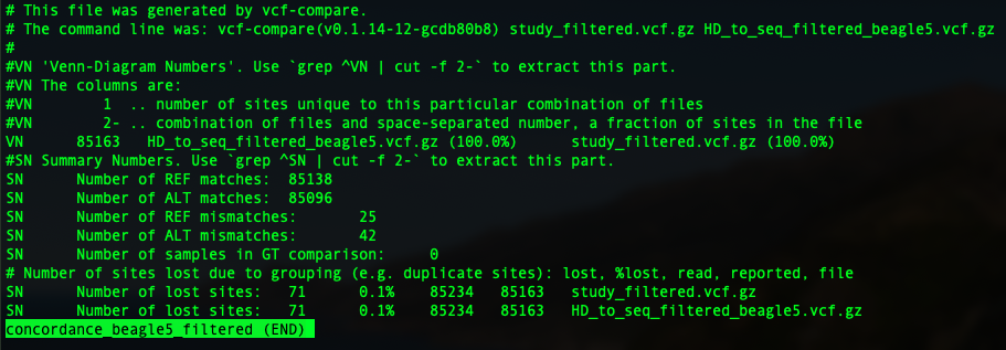
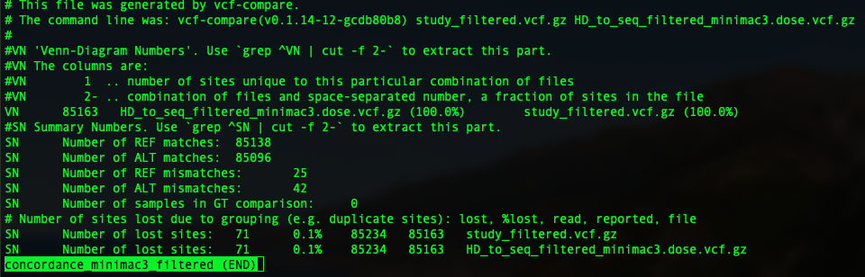
To compare two vcfs and have an idea of genotype concordance, there is a sub-function from vcftools: vcf-compare. so just pop in vcf-compare VCF1 VCF2 > output. You will have an output file.

In the previous session, we have four imputation outputs using both Beagle 5 and minimac3, to impute to filtered and unfiltered sequence reference. So four concordance file will be generated as below:

code

vcf-compare study_filtered.vcf.gz HD_to_seq_filtered_beagle5.vcf.gz > concordance_beagle5_filtered
less concordance_beagle5_filtered

code

vcf-compare study_filtered.vcf.gz HD_to_seq_nonfiltered_beagle5.vcf.gz > concordance_beagle5_nonfiltered
less concordance_beagle5_nonfiltered

code

vcf-compare study_filtered.vcf.gz HD_to_seq_filtered_minimac3.dose.vcf.gz > concordance_minimac3_filtered
less concordance_minimac3_filtered

code

vcf-compare study_filtered.vcf.gz HD_to_seq_nonfiltered_minimac3.dose.vcf.gz > concordance_minimac3_nonfiltered
less concordance_minimac3_nonfiltered

10. Evaluate the performance of imputation: allelic/dosage R-square¶

To calculate the dosage R-square, beagle 5 does not provide a seperate file. You may need a bit code to extract the information:

code

bcftools query -f '%CHROM\t%POS\t%ID\t%REF\t%ALT\t%QUAL\t%FILTER\t%DR2\t%AF\t%IMP\n' HD_to_seq_filtered_beagle5.vcf.gz > HD_to_seq_filtered_beagle5.r2
bcftools query -f '%CHROM\t%POS\t%ID\t%REF\t%ALT\t%QUAL\t%FILTER\t%DR2\t%AF\t%IMP\n' HD_to_seq_nonfiltered_beagle5.vcf.gz > HD_to_seq_nonfiltered_beagle5.r2

The columns of the file we generated are chromosome, position, SNP name, reference allele, alternative allele, quality, filter, dosage r-square, allele frequency, whether it is imputed. It is a thoughtful enough file that provides us all the information, the only additional part we may need to do is calculate the minor allele frequency from allele frequency.

code

head HD_to_seq_filtered_beagle5.r2

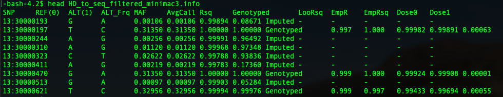
minimac3 generates an info file after it finishes imputing. It is pretty thoughtful that it provides us the minor allele frequency directly. The troubling part is that we have to extract the position from the SNP column for future comparison.

code

head HD_to_seq_filtered_minimac3.info

So we have four output here, and we are going pop them in R to have a look:

R

We either use R at the terminal, or you can use the RStudio associated with Jupyter. When plotting at a terminal, you will need to write the output to a file and open the image from the Jupyter file directory on the left.

The first step is to read in all our output files in R

code

setwd("~/imputation_workshop/imputation")
filteredBG5 <- read.table("HD_to_seq_filtered_beagle5.r2")
nonfilteredBG5 <- read.table("HD_to_seq_nonfiltered_beagle5.r2")
filteredminimac3 <- read.table("HD_to_seq_filtered_minimac3.info", header=T)
nonfilteredminimac3 <- read.table("HD_to_seq_nonfiltered_minimac3.info", header=T)

Then we need to extract all the positions. This step is a bit redundant for beagle outputs but really helpful for the minimac3 output. The function we are gonna use is substr, it tells R to just extract the string from the 4^th digit to the 11^th digit.

code

filteredBG5$Pos <- filteredBG5$V2
nonfilteredBG5$Pos <- nonfilteredBG5$V2
filteredminimac3$Pos <- substr(filteredminimac3$SNP, 4, 11)
nonfilteredminimac3$Pos <- substr(nonfilteredminimac3$SNP, 4, 11)

The next step is to extract the R-square for beagle 5. Usually, it shouldn't be a problem, you get the number in that column directly. However, in this session, we used the unfiltered reference, which contains the multi-allelic positions. In this case, Beagle will give you multiple possible solutions for those multi-allelic positions. In this case, we just take the first solution to make things easier. Here you may see a warning message mentioned NA generated. Don't worry about that.

code

filteredBG5$DR2_filtered_BG5 <- filteredBG5$V8
nonfilteredBG5$DR2_nonfiltered_BG5 <- as.numeric(substr(nonfilteredBG5$V8, 1, 4))
filteredminimac3$Rsq_filtered_minimac3 <- filteredminimac3$Rsq
nonfilteredminimac3$Rsq_nonfiltered_minimac3 <- nonfilteredminimac3$Rsq

Now let's merge both the output files from Beagle and Minimac3, then final merge them into a file called finalmerge

code

mergedBeagle <- merge(filteredBG5, nonfilteredBG5, by.x="Pos", by.y="Pos", all=FALSE)
mergedMinimac3 <- merge(filteredminimac3, nonfilteredminimac3, by.x="Pos", by.y="Pos", all=FALSE)
finalmerge <- merge(mergedBeagle, mergedMinimac3, by.x="Pos", by.y="Pos", all=FALSE)

Let's have a look at the summary

code

summary(finalmerge$DR2_filtered_BG5)
summary(finalmerge$DR2_nonfiltered_BG5)
summary(finalmerge$Rsq_filtered_minimac3)
summary(finalmerge$Rsq_nonfiltered_minimac3)

In both cases of beagle 5 and minimac3, using unfiltered reference gave us poorer performance compared to the filtered ones. Minimac3 gave slightly higher allelic square compare to beagle5. It is not always the case since we are only using 5MB here. And also the performance depends on a lot of parameters. As I mentioned, Beagle is fast but computationally demanding. Minimac 3 is slower but very efficient. There are of course other software for you to choose. Which software to use, what parameters for QC, questions such as those I may not have an answer, you have to figure it out by doing experiments.

As I also mentioned allelic/dosage-r square is a good parameter for evaluating the performance. Here you can see the relationship between MAF and allelic/dosage-r square.

code

plot(finalmerge$MAF.x,finalmerge$DR2_filtered_BG5, pch=4)

code

plot(finalmerge$MAF.x,finalmerge$Rsq_filtered_minimac3, pch=4)

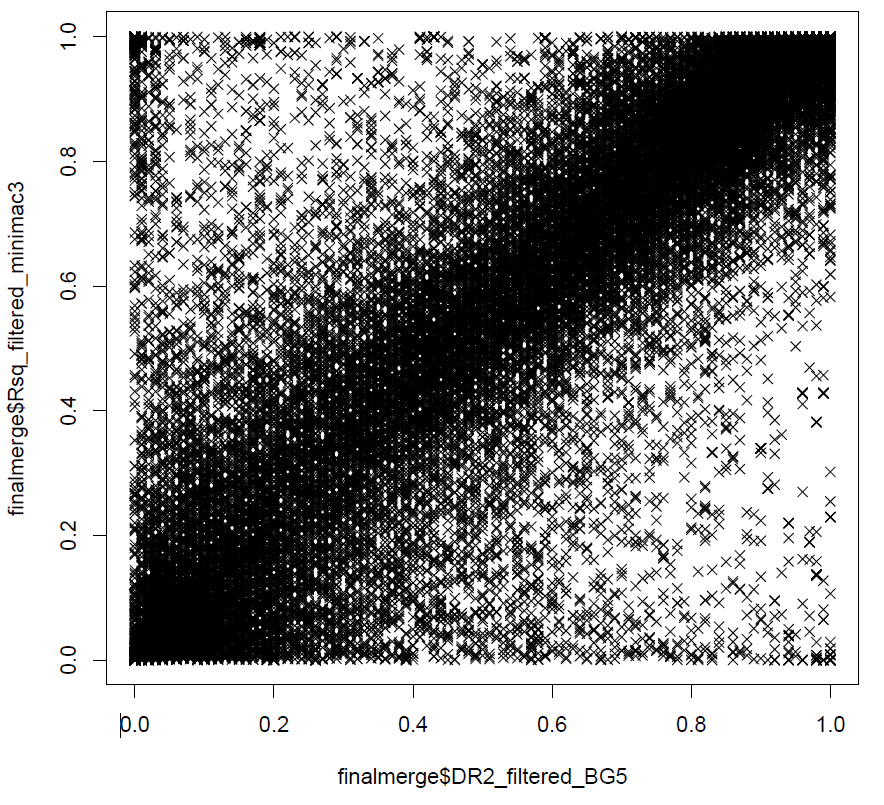
And also, we can also have a look at the correlation between the allelic/dosage-r square from beagle 5 and minimac3.

code

plot(finalmerge$DR2_filtered_BG5,finalmerge$Rsq_filtered_minimac3, pch=4)

Now let's have a look at the poorly imputed regions, the simple way will be just use the position as X-axis and accuracy as Y-axis. The command will be just

code

plot(finalmerge$Pos,finalmerge$DR2_filtered_BG5)
plot(finalmerge$Pos,finalmerge$DR2_nonfiltered_BG5)
plot(finalmerge$Pos,finalmerge$Rsq_filtered_minimac3)
plot(finalmerge$Pos,finalmerge$Rsq_nonfiltered_minimac3)

Since we have large numbers of snps in this region, it will be easier to use a bin plot other than just scatter plots. ggplot2 has a number of functions that are useful for visualising dense data, and we will use geom_hex(). You don't need to run this part for yourself.

code

library(ggplot2)
ggplot(finalmerge,aes(x=Pos,y=DR2_filtered_BG5)) + geom_hex()
ggplot(finalmerge,aes(x=Pos,y=DR2_nonfiltered_BG5)) + geom_hex()
ggplot(finalmerge,aes(x=Pos,y=Rsq_filtered_minimac3)) + geom_hex()
ggplot(finalmerge,aes(x=Pos,y=Rsq_nonfiltered_minimac3)) + geom_hex()

Additional Plots for interest looking at Imputation Accuracy

code

ggplot(finalmerge,
   aes(x=DR2_filtered_BG5,y=Rsq_filtered_minimac3, colour = Pos)) +
  geom_jitter(alpha = 0.2, width = 0.01) +
  labs(x = expression(paste("Beagle5 (",R^{2},")")),
   y = expression(paste("Minimac3 (",R^{2},")")),
   title = "Genotype Accuracy Comparison",
   subtitle = expression(paste(R^{2}," between Minimac3 and Beagle5"))
  ) +
  theme_bw()

# Venn Diagram
#install.packages("ggvenn")
library("ggvenn")

list_venn <- list(Beagle5 = which(finalmerge$DR2_filtered_BG5 >= 0.9),
              Minimac3 = which(finalmerge$Rsq_filtered_minimac3 >= 0.9))
ggvenn(list_venn, c("Beagle5", "Minimac3"))